DynaWind — User Manual

Version: Draft (generated from provided GUI screenshots) • Publisher: WindFast • Status: Professional HTML manual for online publishing

What this manual contains

(1) A clear introduction to the DynaWind workflow, (2) a very detailed field‑by‑field guide describing what to enter in each text box and what each button does, and (3) a complete tutorial example for the 62 m building near Toronto shown in the screenshots.

How to use the screenshots

Every key page includes the exact GUI screenshot used to prepare this guide. You can click any image to zoom, which is helpful when reading labels and verifying what you see in your installed version.

Dyna‑AI Helper

The Dyna‑AI Helper is an embedded assistant intended to reduce user friction and prevent mistakes. It can interpret what DynaWind is showing you, explain what an input means, and help you decide what to enter. It is especially valuable when you are (a) onboarding to the workflow, (b) working with a new site/geometry, or (c) troubleshooting unexpected outputs.

Dyna‑AI Helper can help with:

Field interpretation — explain what any text box/parameter represents (units, typical ranges, and consequences).
Input recommendation — suggest reasonable starting values based on building height, site region, and analysis intent.
Data sanity checks — spot obvious inconsistencies (e.g., units mixups, unrealistic roughness, wrong wind direction conventions).
Results explanation — interpret plots/tables, define key metrics (e.g., return period mapping, spectra), and identify red flags.
Workflow guidance — tell you what to do next and what outputs should appear if the step was successful.
Troubleshooting — suggest causes and fixes (mesh quality, coordinate issues, missing files, solver settings).

Practical examples:

If you are unsure what to enter for z0M (roughness length), Dyna‑AI can explain typical values by land‑use category and how that impacts the inlet profile.
If a force spectrum looks noisy, Dyna‑AI can explain whether you need longer sampling, how Nignore_end affects statistics, and what stability indicators to check.
If a solver run stops early, Dyna‑AI can interpret the solver log and propose parameter adjustments or file checks.

In this manual, the Dyna‑AI Helper is referenced as a recommended companion at every step where users typically need judgment.

Projects & file management

DynaWind organizes all inputs and outputs into a project directory. This is essential for reproducibility, collaboration, and reporting. A project typically contains: (1) saved input parameters, (2) geometry and mesh assets, (3) solver outputs and logs, (4) post‑processed results (tables/figures), and (5) exports/reports.

Top bar actions

Control	What it does	When to use
Project Directory (path field)	Selects where DynaWind will create and save the project folder and all outputs.	First step for a new job. Use a dedicated folder per project and keep it backed up.
Create Project	Creates a new project folder structure and initializes the project state.	Use when starting a new site/building.
Load Project	Loads an existing project and restores saved input values and file links.	Use to continue work or review results.
Save Project	Saves current inputs and relevant state to the project directory.	Use often—after completing each major step.
View Results	Opens saved result views/tables/figures for the project.	Use after Climate/Terrain/Solver/Scaling steps.
Export Dyna / Import Dyna	Exports or imports a packaged DynaWind project bundle for sharing/archiving.	Use for collaboration, submission, or moving the project between machines.
Generate Report	Compiles a report package from the project data (inputs + outputs).	Use once your workflow is complete (or for interim milestones).

Tip: Keep naming consistent. DynaWind often uses a Project or output folder name field inside modules—use the same base name across the workflow to avoid mixing outputs.

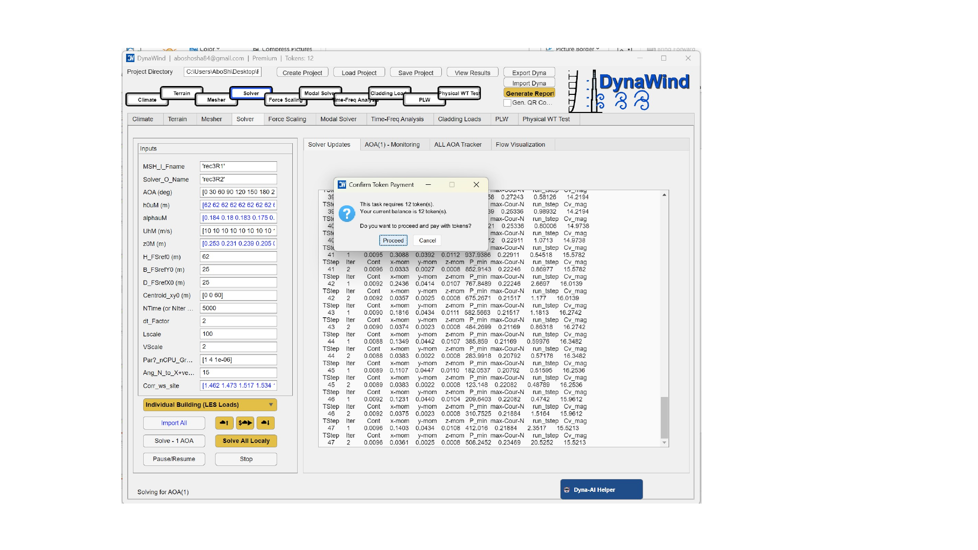
Tokens

Some compute‑intensive operations may require tokens (depending on your license/workflow configuration). When a token‑gated action is triggered, DynaWind prompts you to confirm the token payment before proceeding.

Token confirmation prompt — **Token confirmation example.** Confirm before running an operation that consumes tokens.

Best practices

Validate inputs first (especially meshes and wind directions) before starting token‑consuming computations.
Run one AOA first to confirm the workflow, then batch all AOAs.
If uncertain, use Dyna‑AI Helper to review your setup before proceeding.

2. GUI reference: what to enter and what each button does

This section is organized by the major workflow tabs visible in the main window. For each tab, you will find: (a) a screenshot, (b) a field‑by‑field explanation (meaning, units, typical values, and notes), and (c) button behavior and expected outputs.

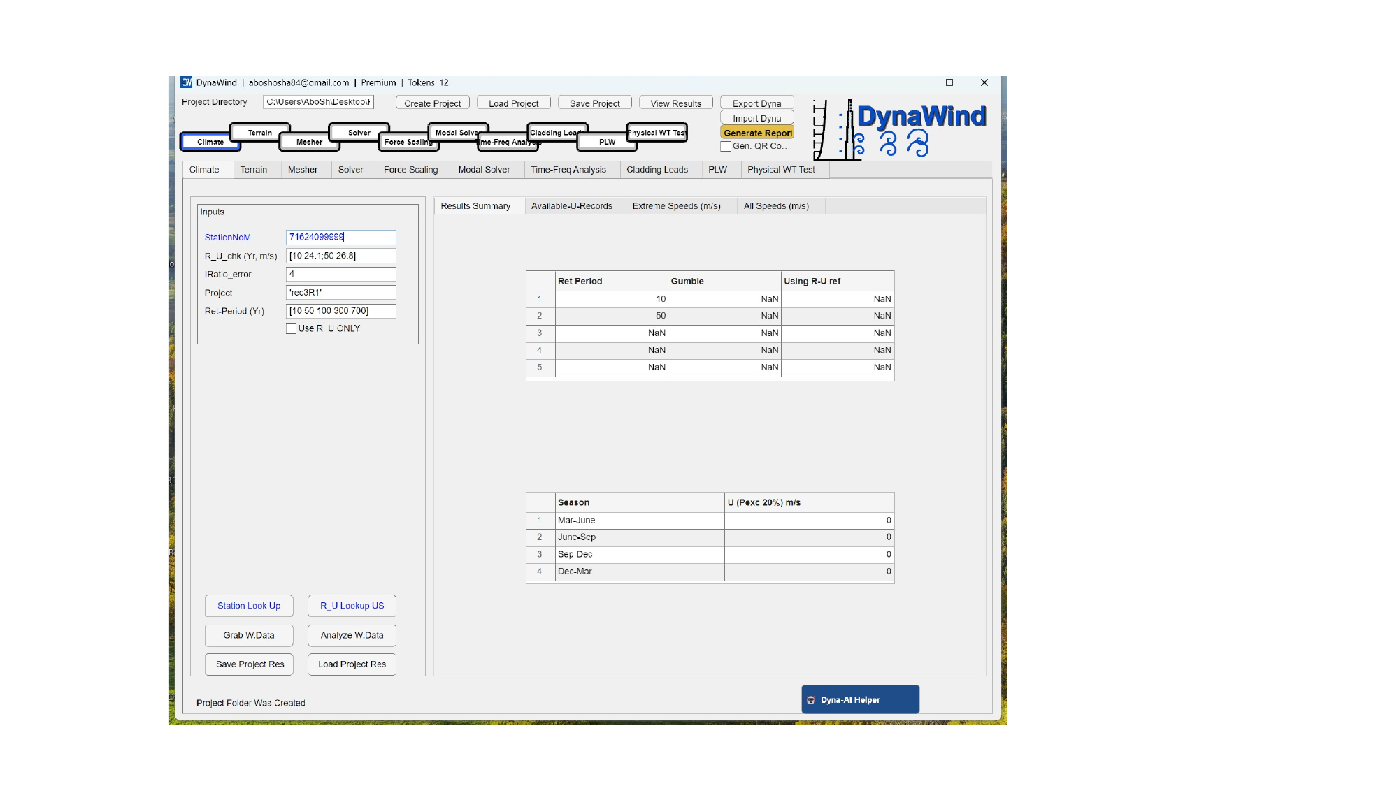
2.1 ClimateWorkflow Step 1/10

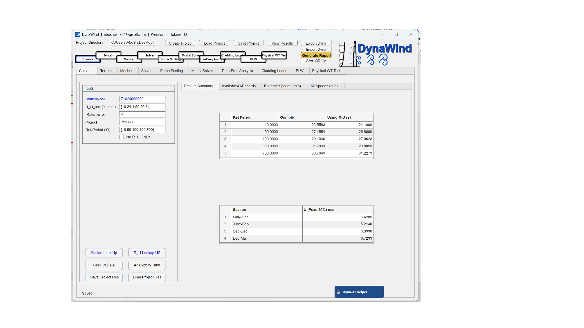
The Climate tab is where you connect your project to wind climate data: station selection, record processing, return periods, and summarized extreme wind speeds. (see Fig. 2.1).

Climate tab with computed return-period values — **Fig. 2.1 — Climate tab.**

Inputs (left panel)

Field	What to enter	Notes / typical usage
StationNoM	Station identifier used by your dataset source.	Use Station Look Up if you do not know the ID. Keep it consistent for the project.
R_U_chk (Yr, m/s)	A list of check points like `[T U]` pairs (e.g., `[10 24.1; 50 26.8]`).	Used to verify or anchor return‑period mapping against known values or references.
IRatio_error	Integer / scalar tolerance parameter for climate fitting/ratio checks.	Higher values relax screening; lower values enforce stricter fit/consistency. Use Dyna‑AI Helper if unsure.
Project	Project label or internal key (string).	Keep it short and consistent (e.g., `rec3R1`).
Ret‑Period (Yr)	Return periods you want results for, as a list (e.g., `[10 50 100 300 700]`).	These populate the summary tables. Adjust per code/design requirements.
Use R_U ONLY (checkbox)	Enable if you want to bypass record analysis and use only the provided `R_U_chk` mapping.	Useful when you have authoritative site wind speeds and want DynaWind to use them directly.

Buttons

Button	Action	Expected output
Station Look Up	Opens tools to find the correct station identifier for your location.	Station ID shown/selected for entry into `StationNoM`.
R_U Lookup US	Optional lookup utility for US reference mappings (if applicable to your dataset configuration).	Populates a reference mapping to compare against your record processing.
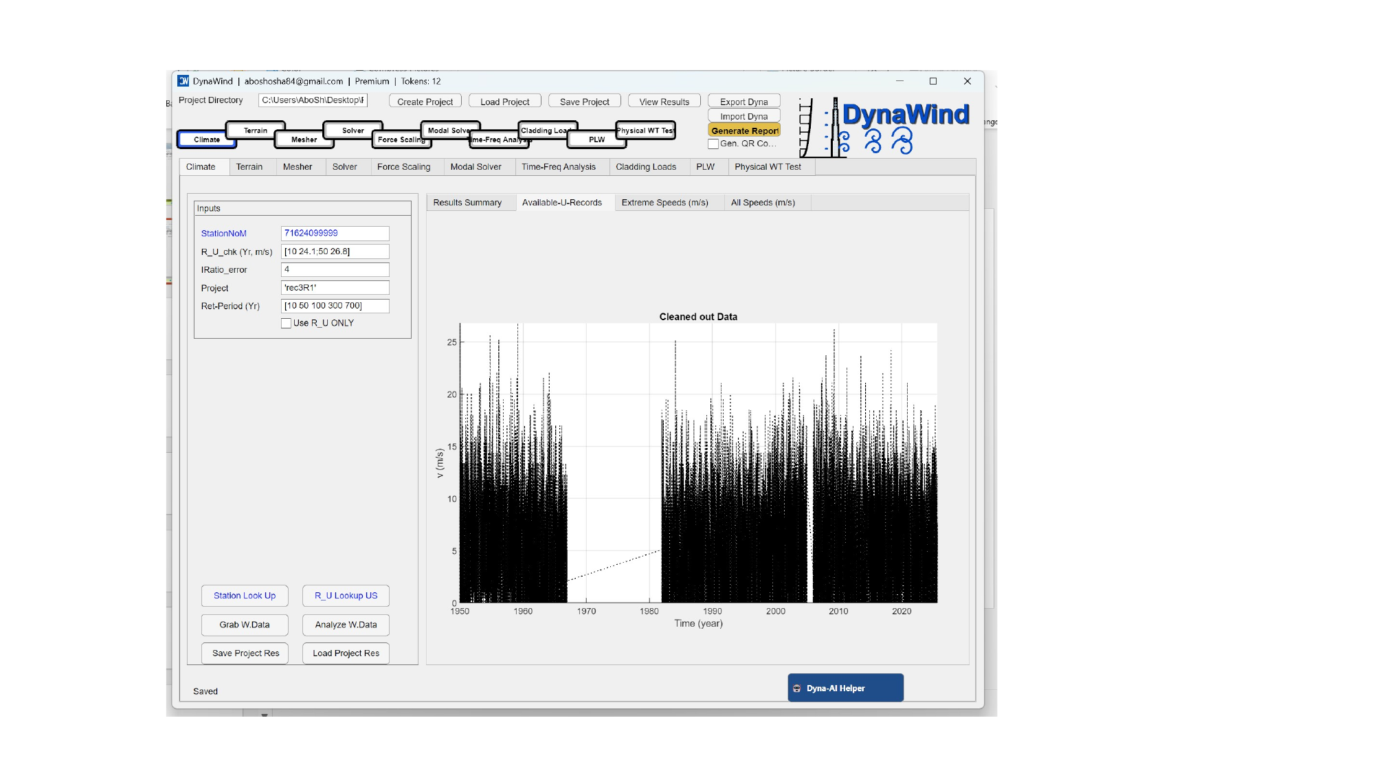
Grab W.Data	Downloads/loads wind data records for the selected station.	Record availability lists and raw series used by analysis.
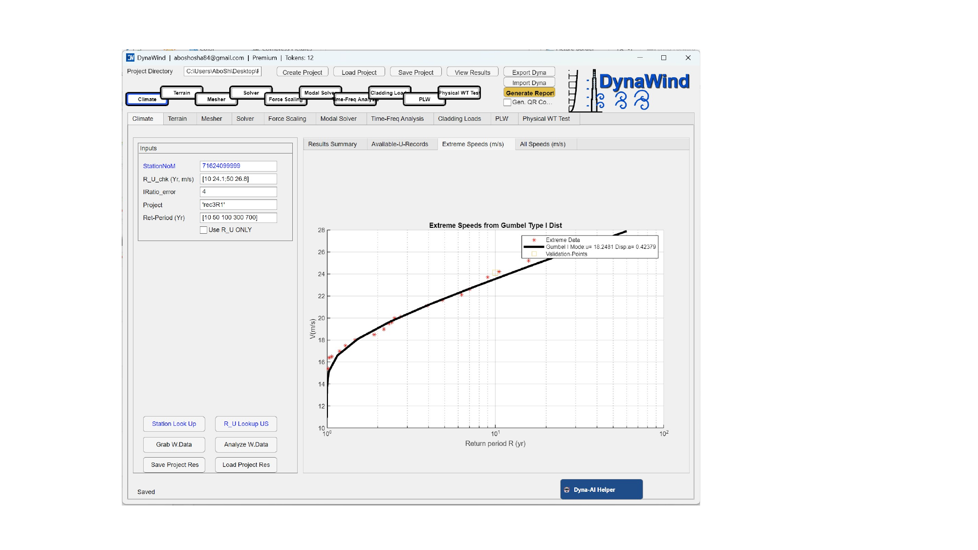
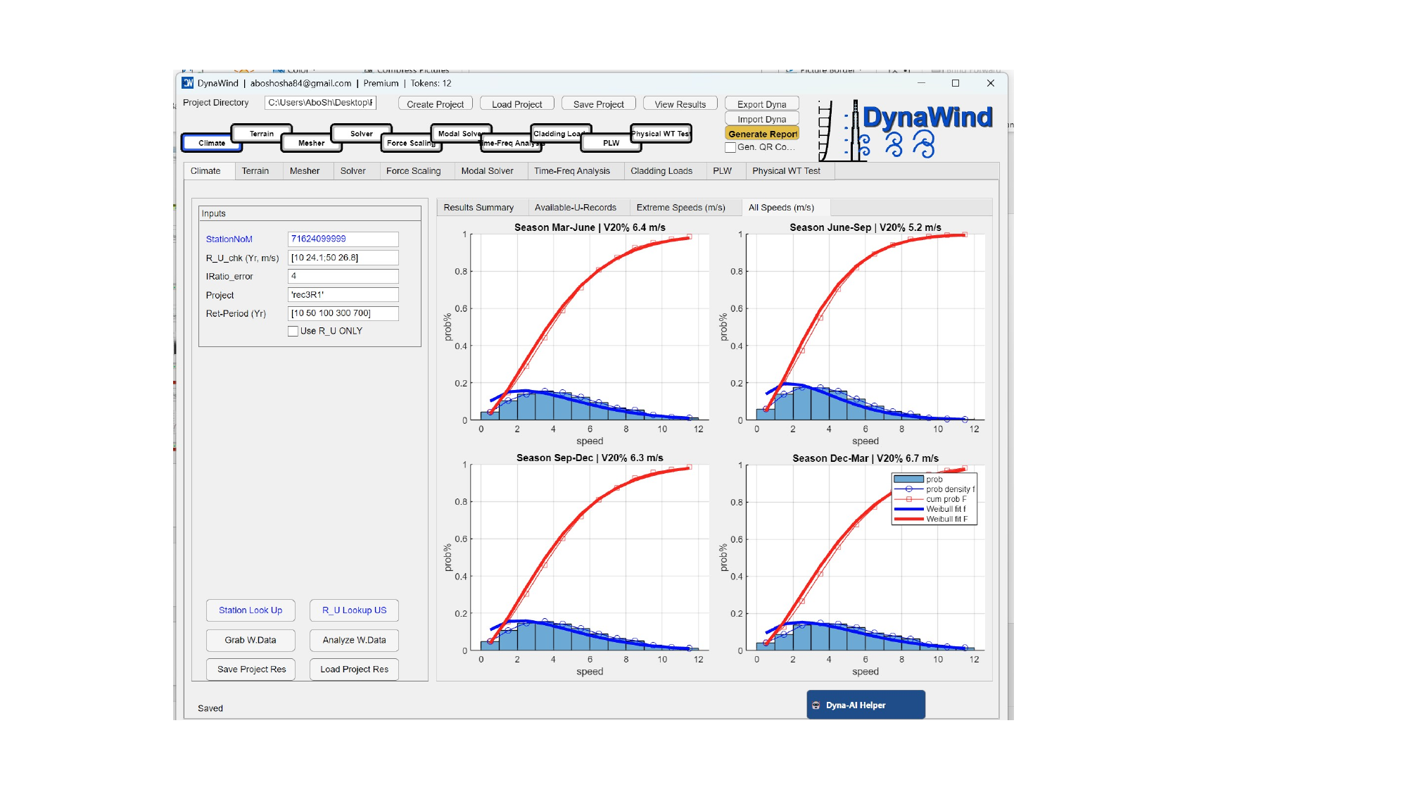
Analyze W.Data	Processes wind records to estimate extremes and return‑period winds (e.g., Gumbel fit).	Return‑period wind speed table and seasonal statistics (if enabled in your build).
Save Project Res	Saves computed climate results to the project directory.	Files that later modules can reference (terrain scaling, force scaling).
Load Project Res	Loads previously saved climate results.	Restores tables without re‑running analysis.

What to check before moving on

Return‑period winds are populated for all target Ret‑Period values.
Values are within a reasonable range for the region; use Dyna‑AI Helper to sanity‑check.
The station location is appropriate for your site (coastal vs inland, elevation, exposure).

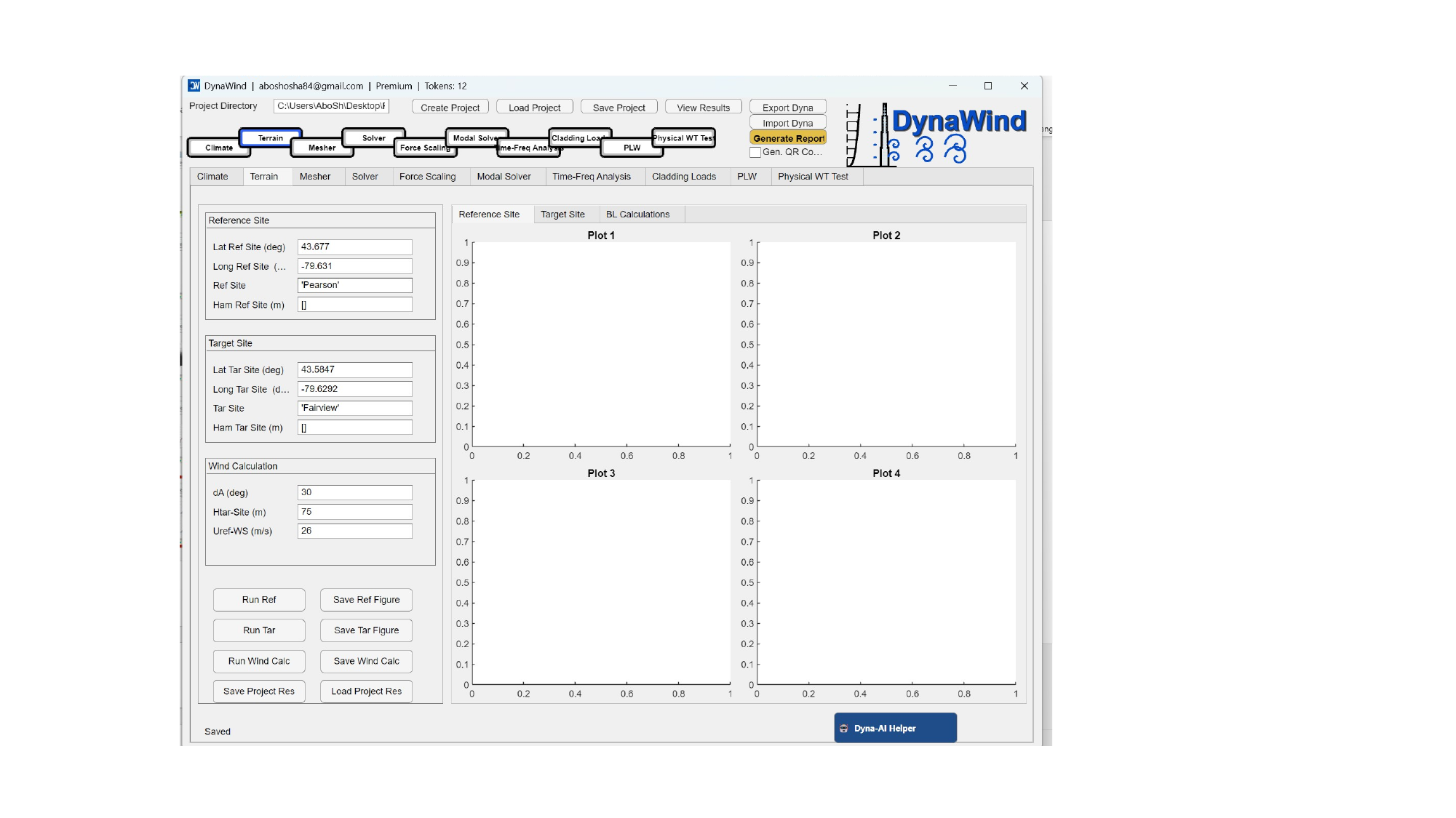
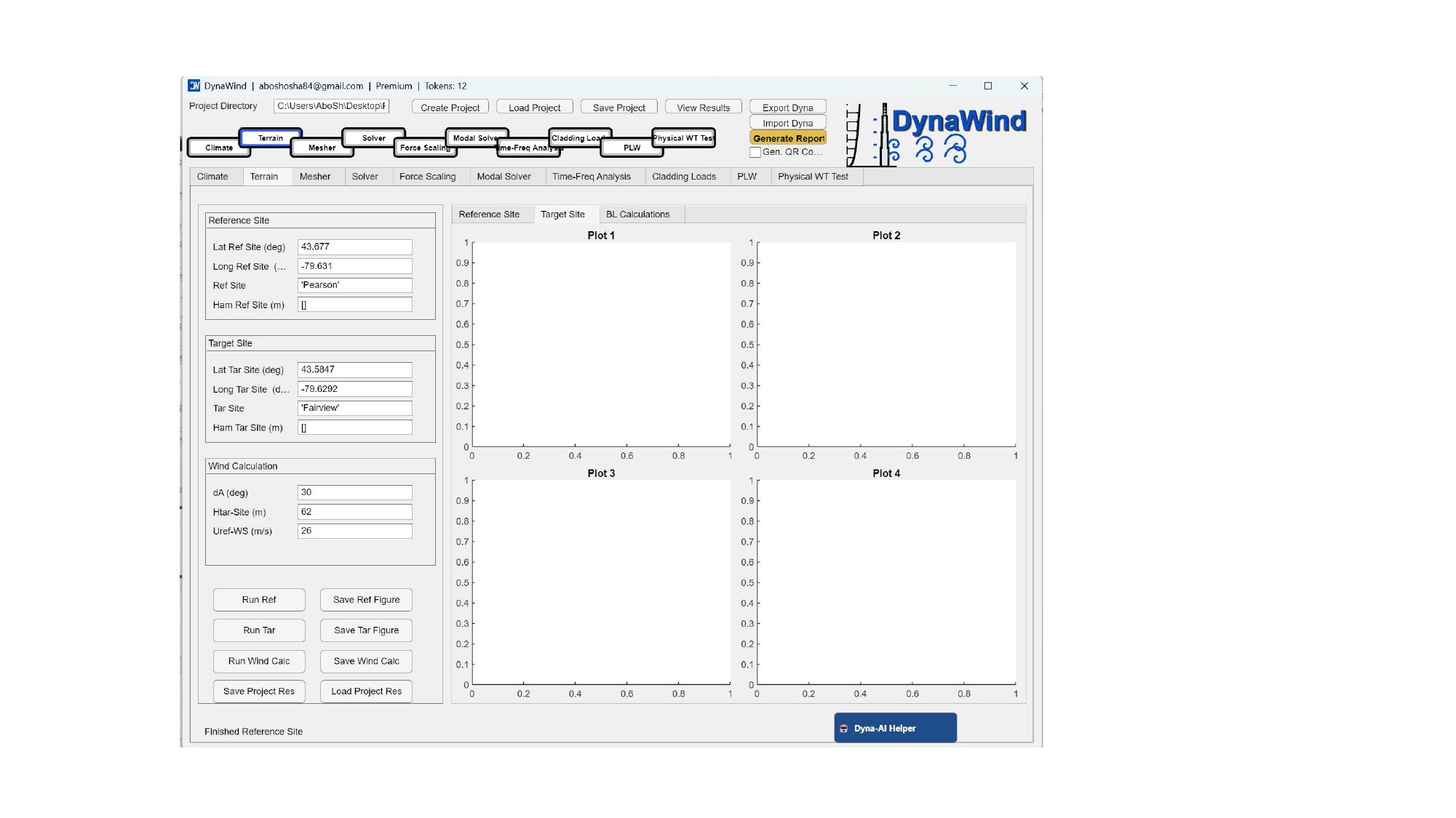
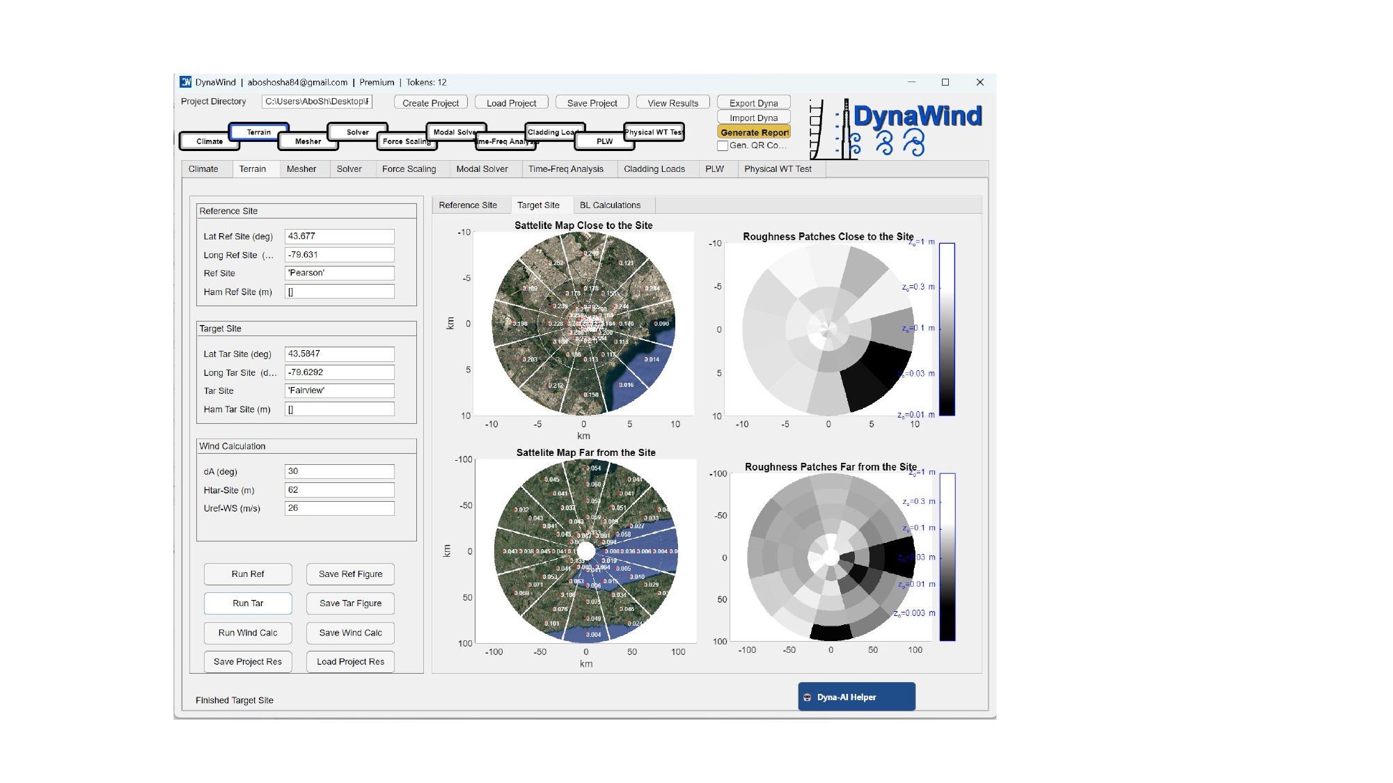
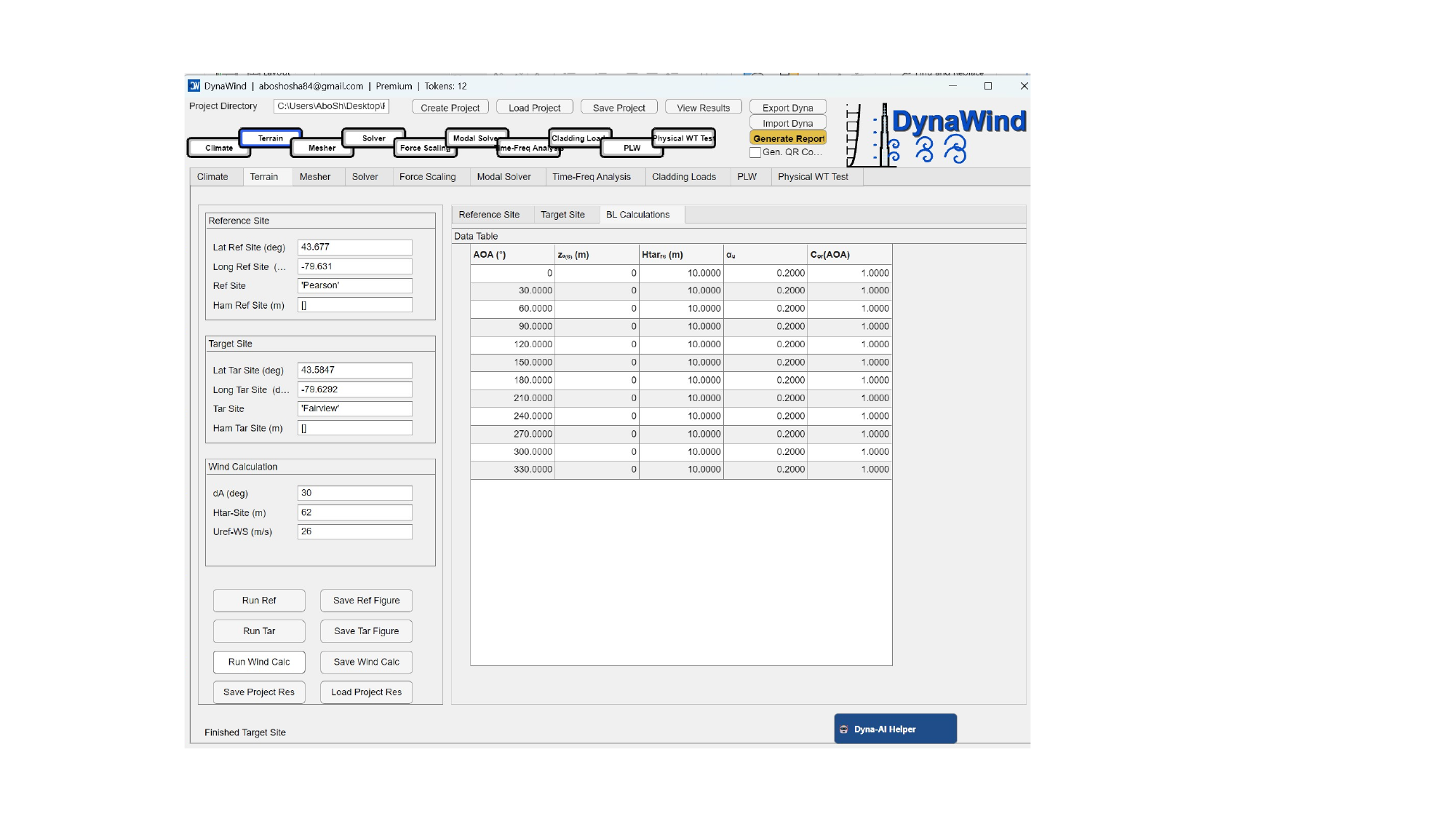
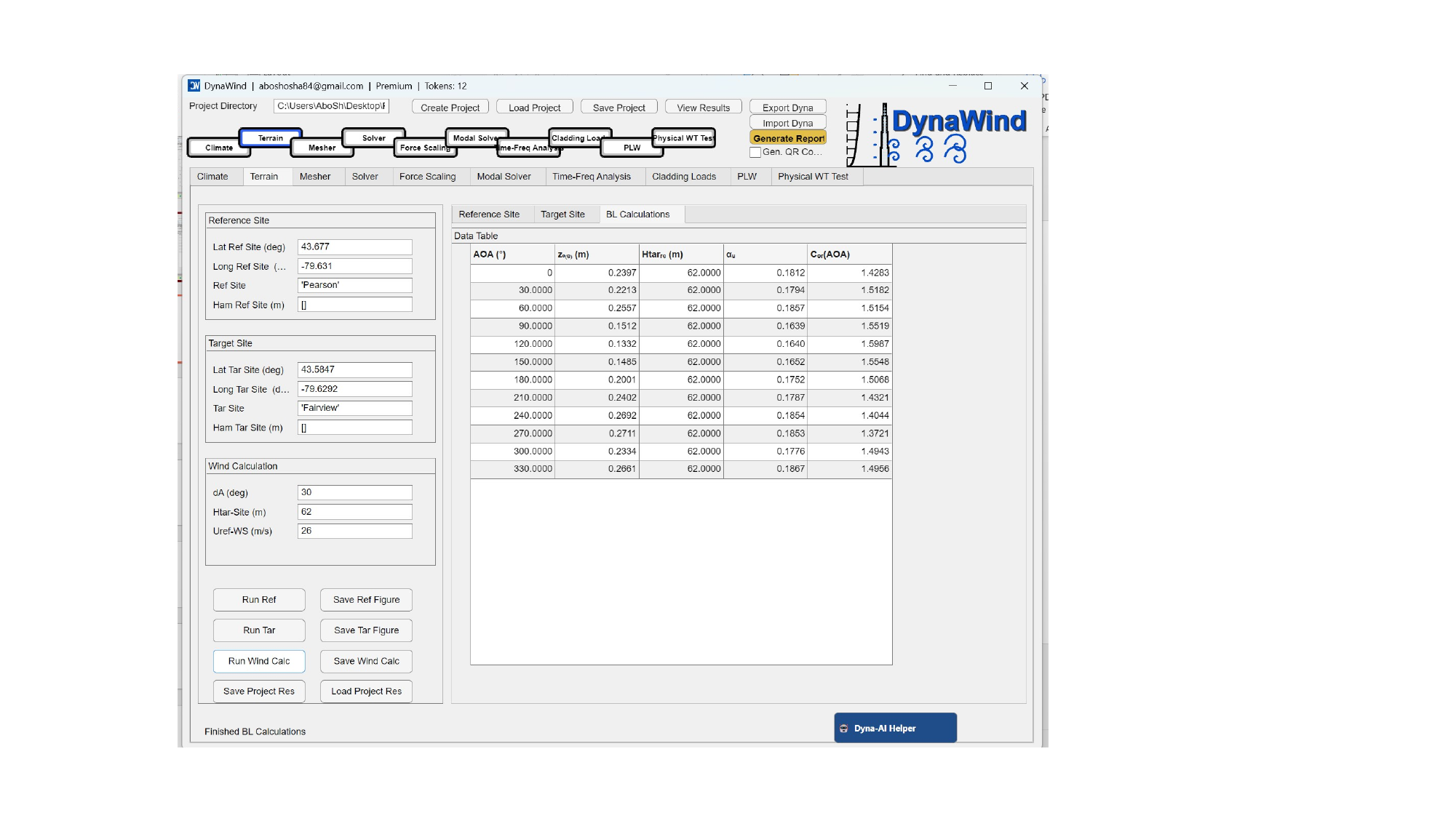
2.2 TerrainWorkflow Step 2/10

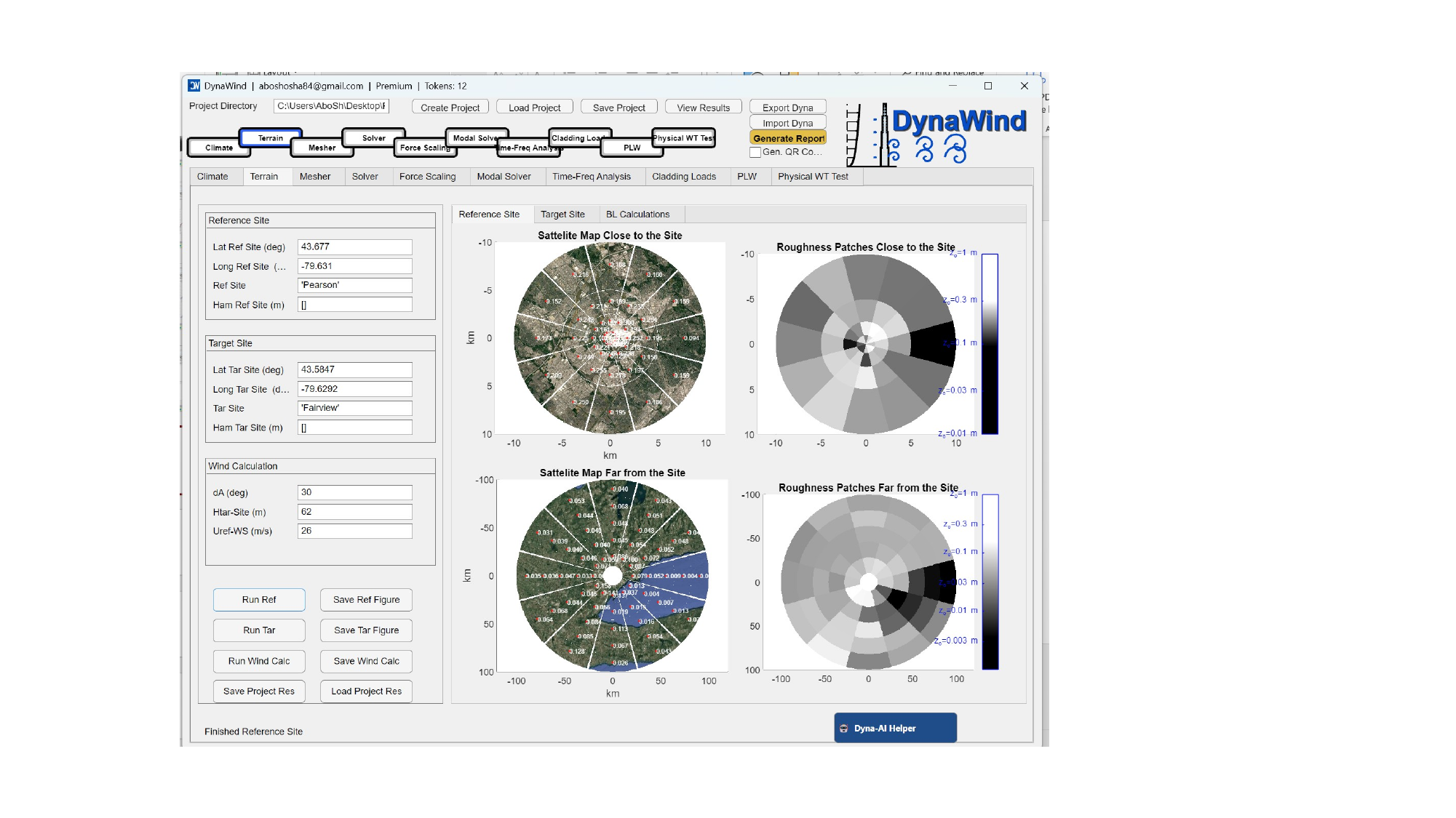
The Terrain tab characterizes the surroundings of your site using roughness patches and exposure mapping. DynaWind distinguishes between near and far surroundings and provides tools to compute corrections for the target site relative to a reference. (see Fig. 2.2).

Terrain tab showing satellite maps and roughness patches — **Fig. 2.2 — Terrain tab.**

Reference Site block

Field	What to enter	Why it matters
Lat Ref Site (deg)	Latitude of the reference site.	Used to fetch/map terrain data around the reference context.
Long Ref Site (deg)	Longitude of the reference site.	Must match the coordinate convention used by your mapping source.
Ref Site	A short label (e.g., neighborhood / city label).	Helps in organizing figures and outputs.
Ham Ref Site (m)	Reference height/elevation parameter (if required by your workflow).	Leave blank if not used; use Dyna‑AI Helper to confirm your build's expectation.

Target Site block

Field	What to enter	Why it matters
Lat Tar Site (deg)	Latitude of the project site.	Defines where roughness patches are extracted.
Long Tar Site (deg)	Longitude of the project site.	Accuracy matters—small location shifts can change local roughness categories.
Tar Site	Short site label (e.g., district name).	Used in saved figures and result filenames.
Ham Tar Site (m)	Target height/elevation parameter (if used).	Optional depending on configuration.

Wind Calculation block

Field	What to enter	Notes
dA (deg)	Angular resolution of sectors (e.g., `30` gives 12 sectors).	Smaller dA gives more directional detail but more processing.
Htar‑Site (m)	Characteristic height at the target site used for exposure evaluation (often building height).	For the tutorial case, this is 62 m.
Uref‑WS (m/s)	Reference wind speed used when forming ratios/corrections.	Often the climate‑derived wind at a chosen return period or reference condition.

Buttons

Button	Action	Expected outputs
Run Ref	Computes terrain/roughness descriptors for the reference site.	Reference site maps and roughness patch distributions.
Run Tar	Computes terrain/roughness descriptors for the target site.	Target site maps and roughness patch distributions.
Run Wind Calc	Computes directional correction factors / exposure adjustments.	Directional corrections that feed force scaling and/or solver inlet setup.
Save Ref Figure/Save Tar Figure	Saves site maps and roughness visuals.	Figures for reporting and QA.
Save Wind Calc	Saves correction factors and related outputs to the project.	Files reused in scaling and later modules.
Save Project Res/Load Project Res	Persists or restores Terrain results.	Skip reprocessing when returning to the project.

Use Dyna‑AI Helper here if:

You are unsure what roughness values mean (z0 interpretation) or how the near/far maps influence the correction.
Your maps show unexpected patch patterns (e.g., water/forest misclassification) and you need a sanity check.

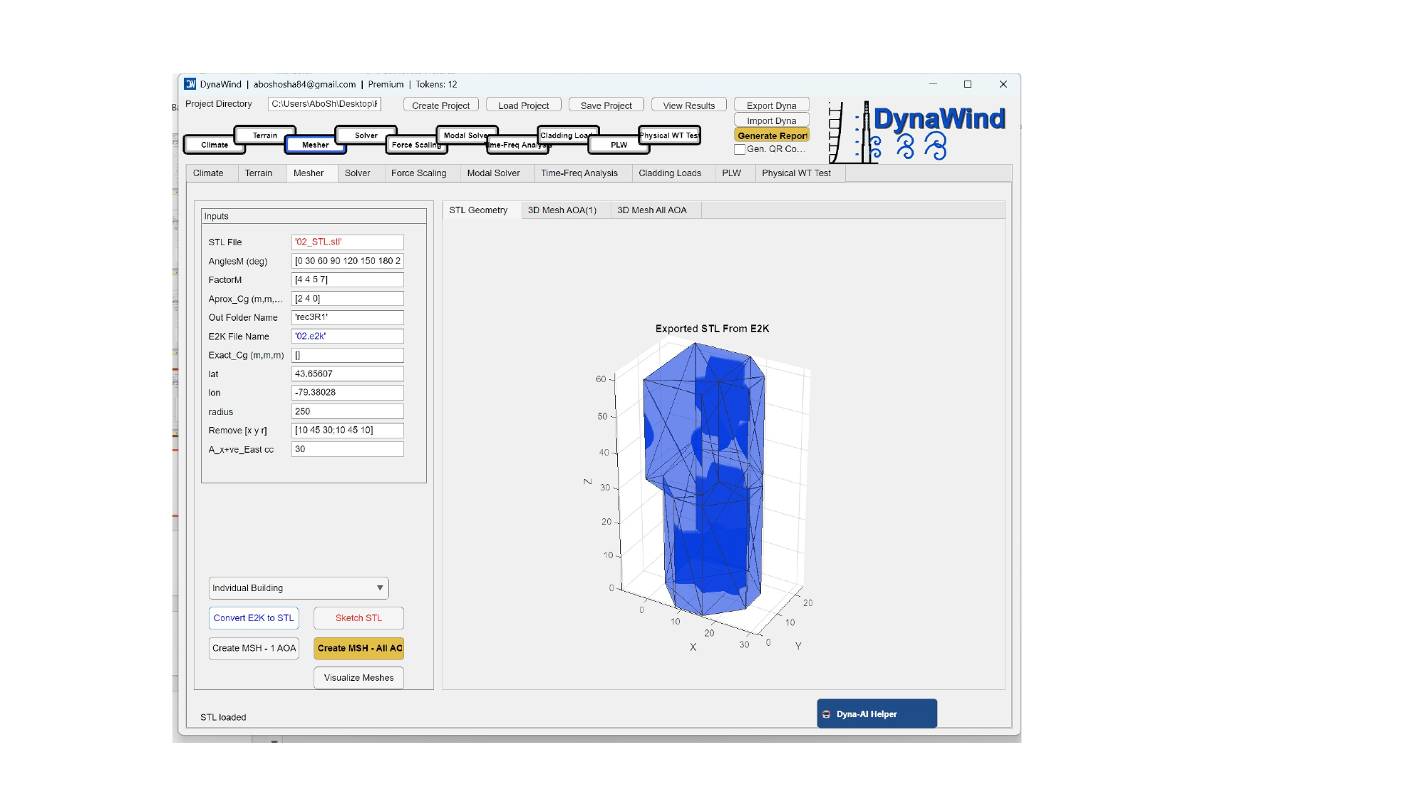
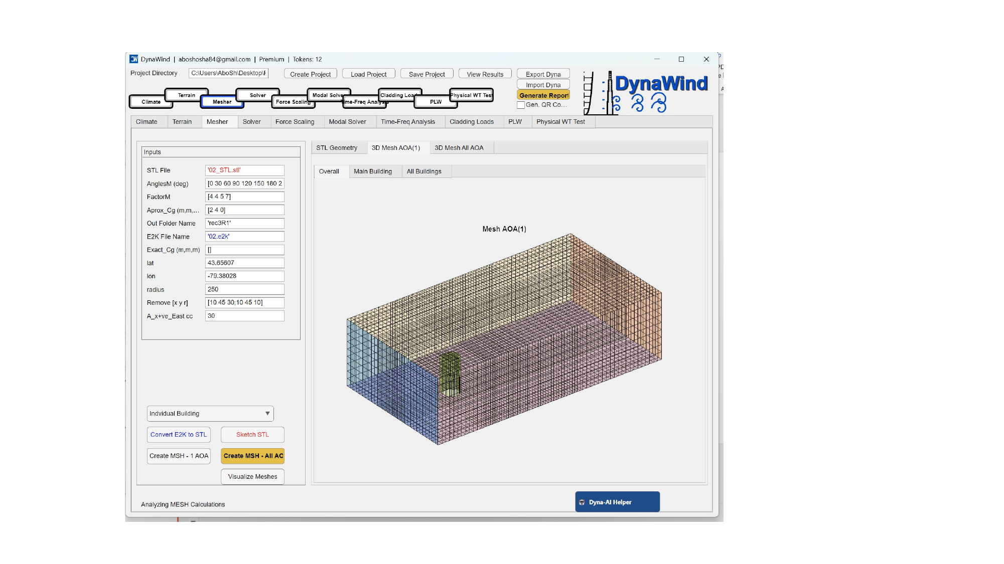
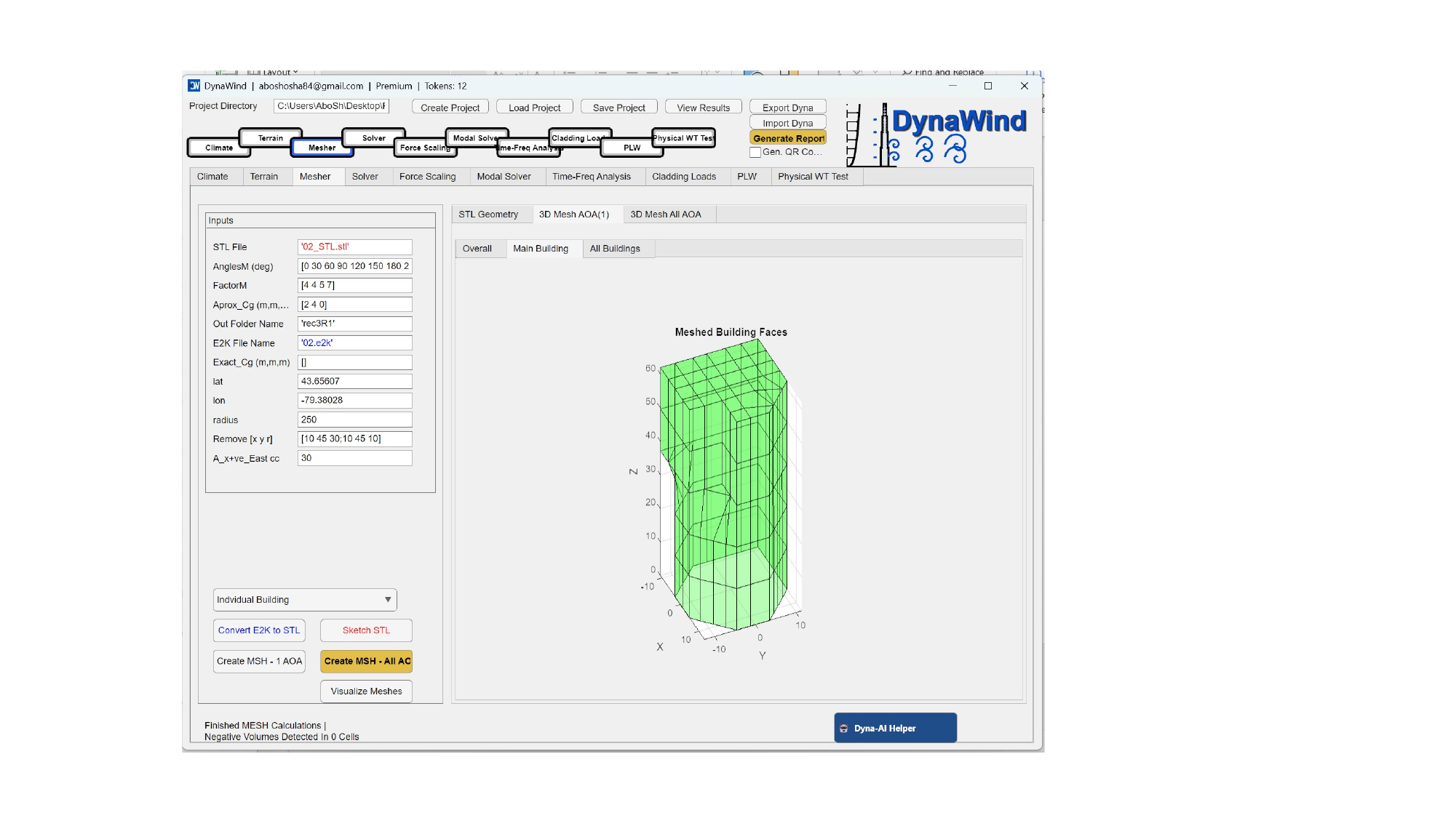
2.3 MesherWorkflow Step 3/10

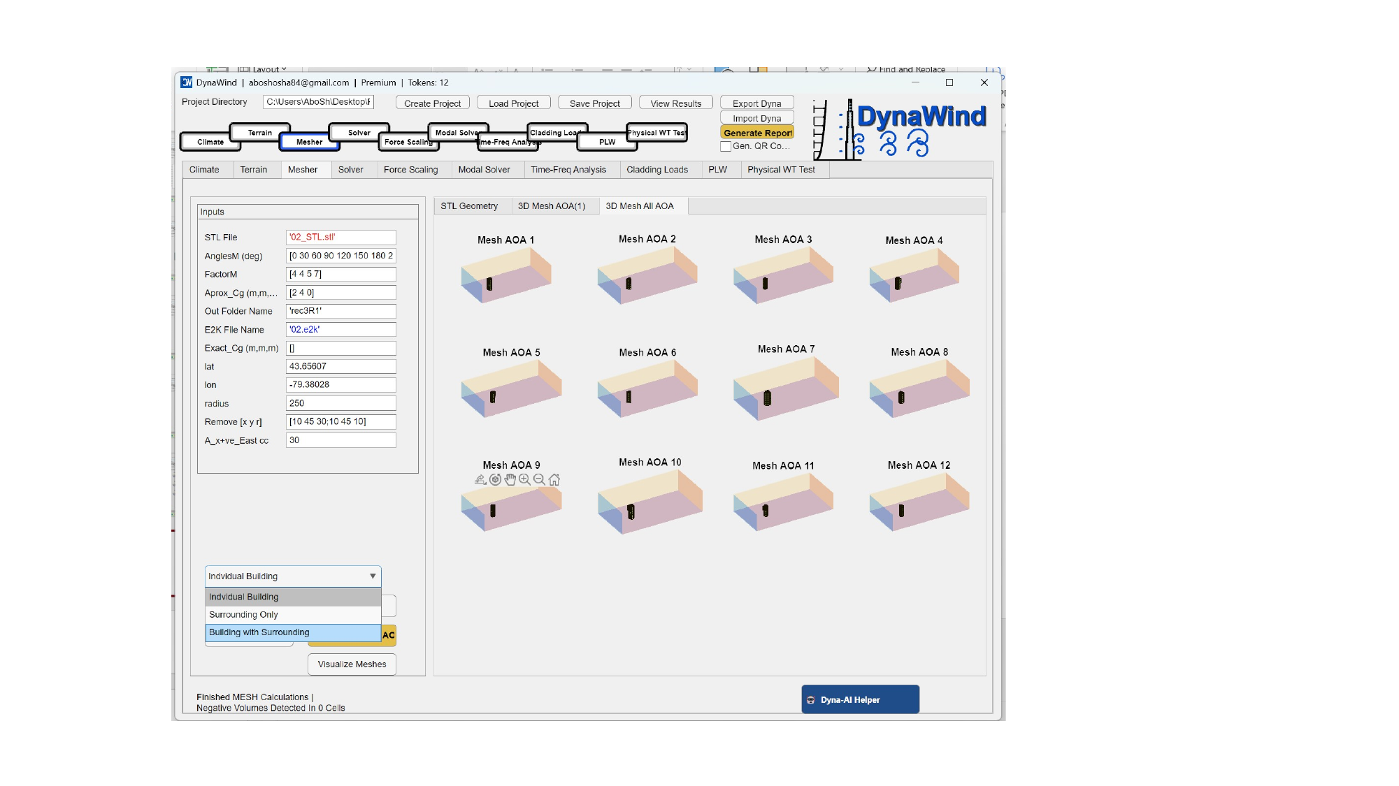
The Mesher tab converts building geometry into the computational representation used by the solver. DynaWind supports direct STL workflows and conversion from structural models (e.g., E2K) into STL. You then define the wind directions (angles of attack), configure meshing factors, and generate one or multiple meshes. (see Fig. 2.3).

Inputs

Field	What to enter	Practical guidance
STL File	STL geometry filename (relative to project folder or full path).	Use a clean watertight STL if possible. If starting from E2K, use conversion below.
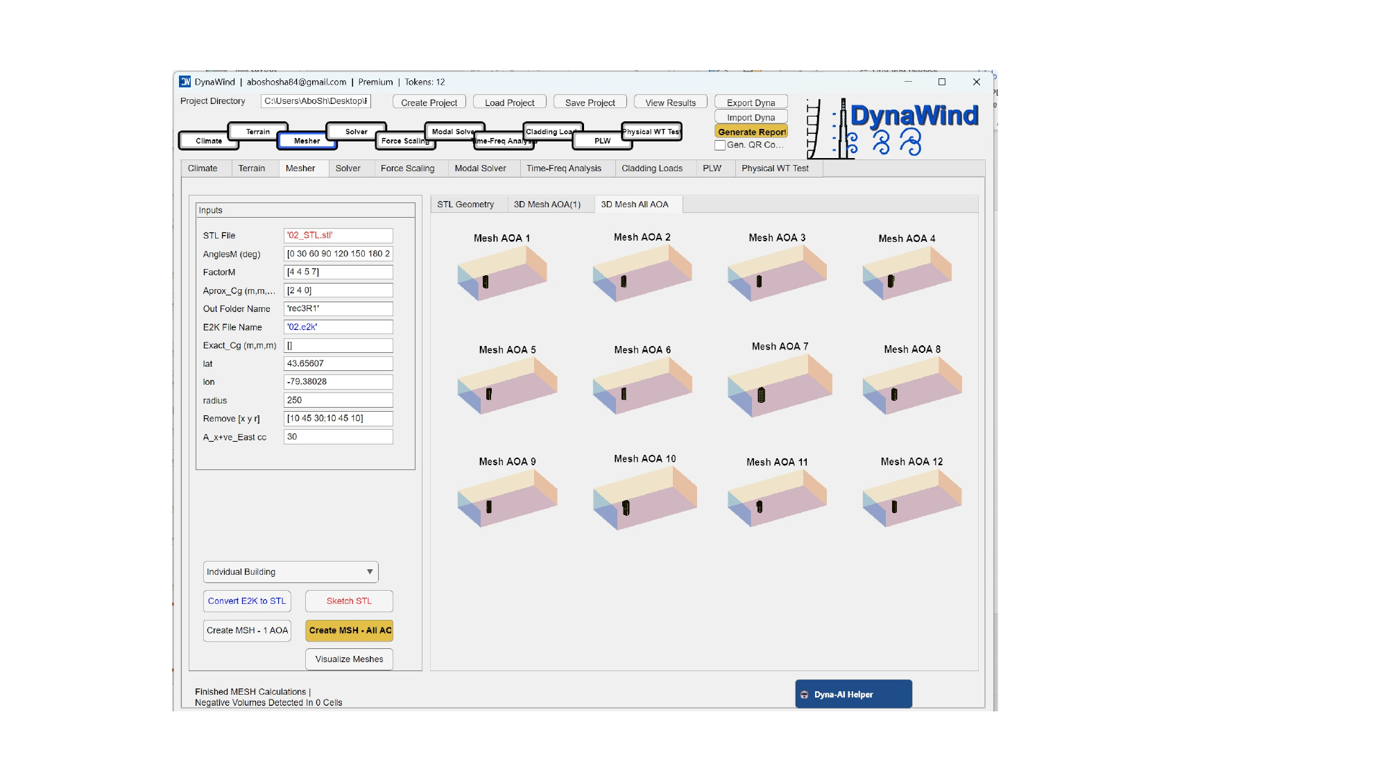
AnglesM (deg)	List of wind directions/angles of attack to run, e.g. `[0 30 60 … 330]`.	Match your terrain sectoring and reporting needs. Start with a coarse set, then refine if required.
FactorM	Meshing factor(s) controlling domain resolution.	Higher = more cells = higher compute cost. Use Dyna‑AI Helper for recommended starting values.
Approx_Cg (m,m,m)	Approximate centroid of geometry in model coordinates.	Used to position the building in the domain; correct values prevent offsets and rotation issues.
Out Folder Name	Output folder key for mesh assets (e.g., `rec3R1`).	Keep consistent across meshing, solver, and scaling.
E2K File Name	Structural model file (e.g., `02.e2k`) used for conversion.	Use when geometry originates from ETABS/SAP export.
Exact_Cg (m,m,m)	Optional override for centroid if known precisely.	Use when you have verified coordinates from CAD/model exports.
lat / lon	Site coordinates used for surroundings (if mesher uses location‑based context).	Should match Terrain tab target site coordinates.
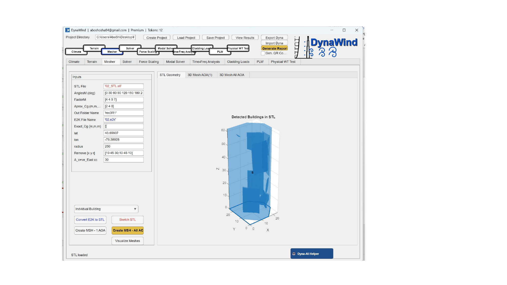
radius	Radius (m) for extracting/including surrounding context, if applicable.	Use a radius that captures relevant nearby buildings/terrain features.
Remove [x y r]	List of removal masks (x,y,r) to exclude problematic geometry areas.	Useful for deleting artifacts or isolating buildings; verify using STL preview.
A_x+ve_East cc	Angle convention offset, defining how AOA relates to East/coordinate axes.	Critical for correct wind direction mapping. Confirm with Dyna‑AI Helper if uncertain.

Mode selector (dropdown)

The dropdown selects which geometry to mesh:

Individual Building — mesh only the main building (fastest, for early checks).
Surrounding Only — mesh only the surroundings (useful for validating context).
Building with Surrounding — full model (recommended for final results).

AOA mesh previews and dropdown — **AOA mesh previews.** DynaWind can generate per‑AOA meshes and display thumbnails for quick QA.

Buttons

Button	Action	What to look for
Convert E2K to STL	Generates an STL geometry from the E2K structural model.	Check that the resulting STL matches the intended building envelope and that axes/origin are correct.
Sketch STL	Provides a quick visualization/preview of the STL geometry.	Use this to detect missing faces, holes, or incorrect scale early.
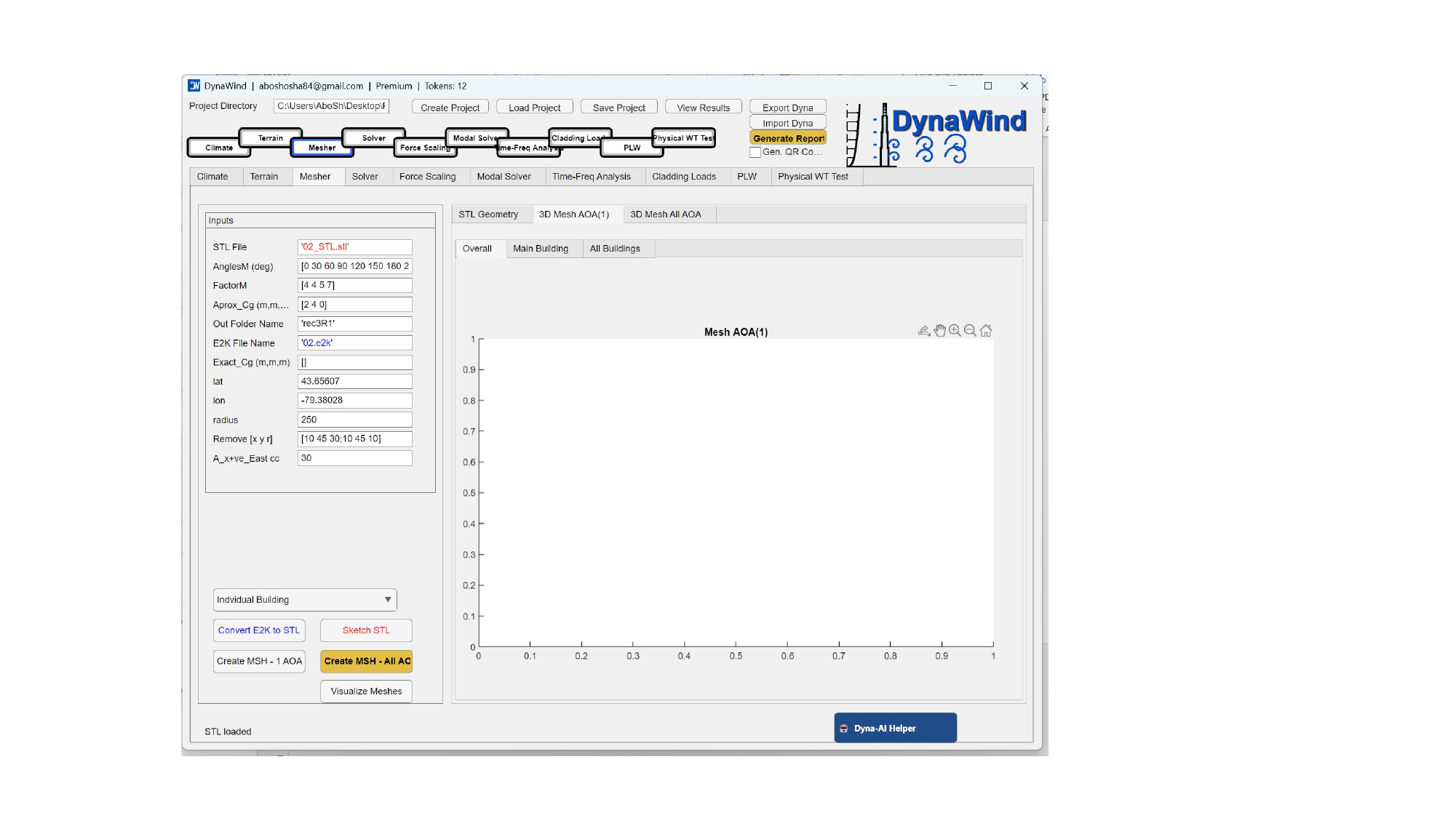
Create MSH – 1 AOA	Generates a mesh for a single AOA (usually the first in the list).	Best practice before running all AOAs—confirm domain, refinement, and geometry placement.
Create MSH – All AO	Generates meshes for all AOAs specified.	Ensure sufficient disk space; this can be compute‑ and storage‑intensive.
Visualize Meshes	Opens mesh visualization for QA.	Look for cell skewness, negative volumes, and adequate refinement near surfaces.

Common pitfalls:

Incorrect AOA convention (clockwise vs counter‑clockwise). Confirm using a simple test wind direction and expected wake location.
Centroid/offset wrong → building appears shifted. Fix using Approx_Cg or Exact_Cg.
Mesh too coarse near edges → unstable forces or poor cladding pressures. Increase refinement via FactorM or module‑specific settings.

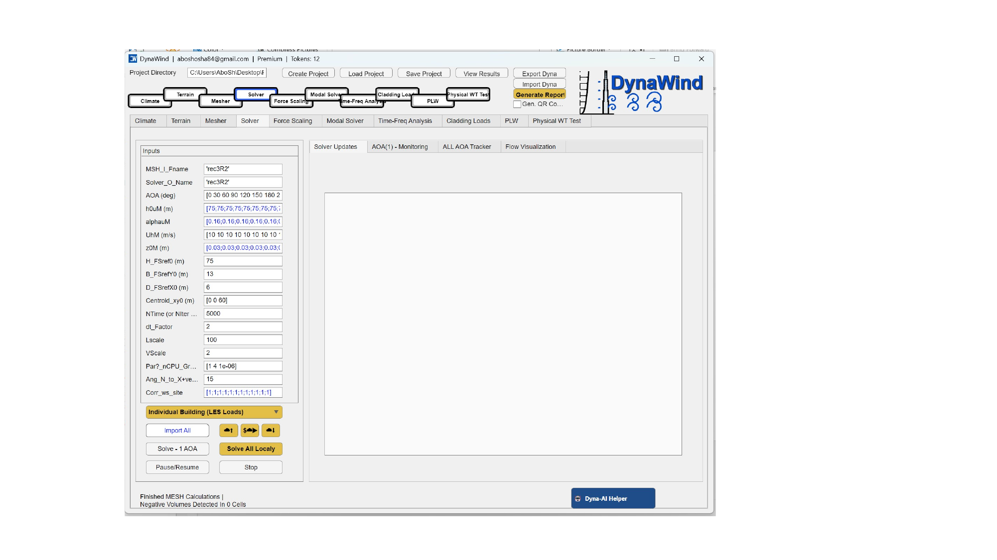
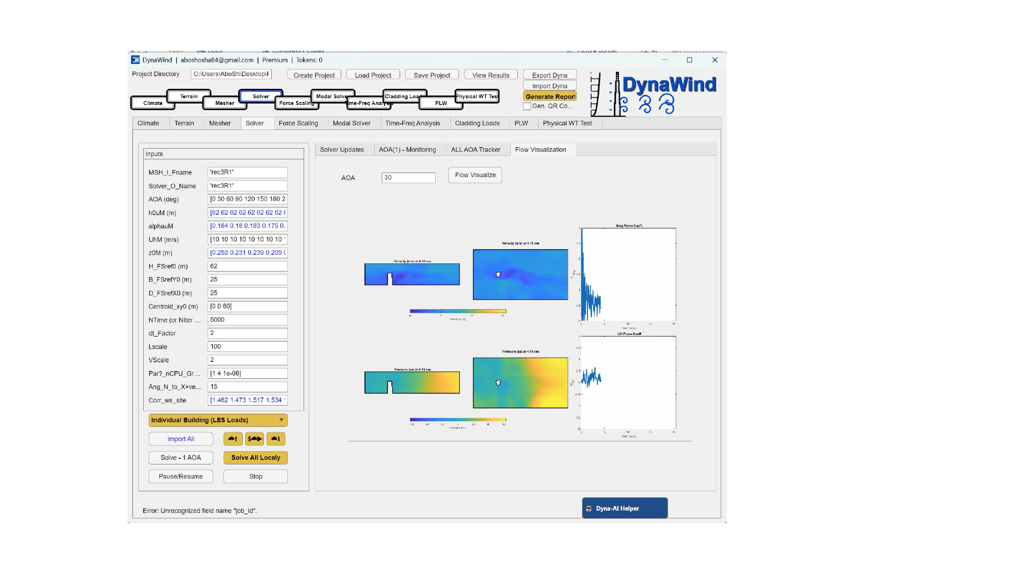
2.4 Solver (LES)Workflow Step 4/10

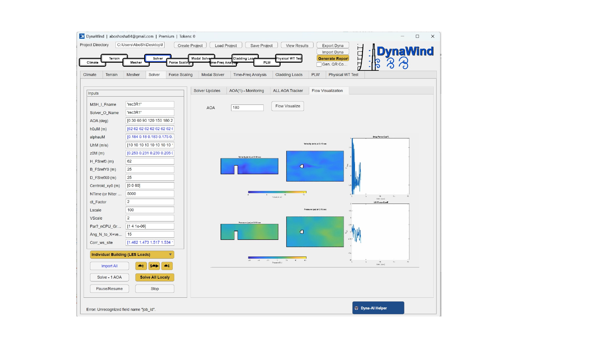
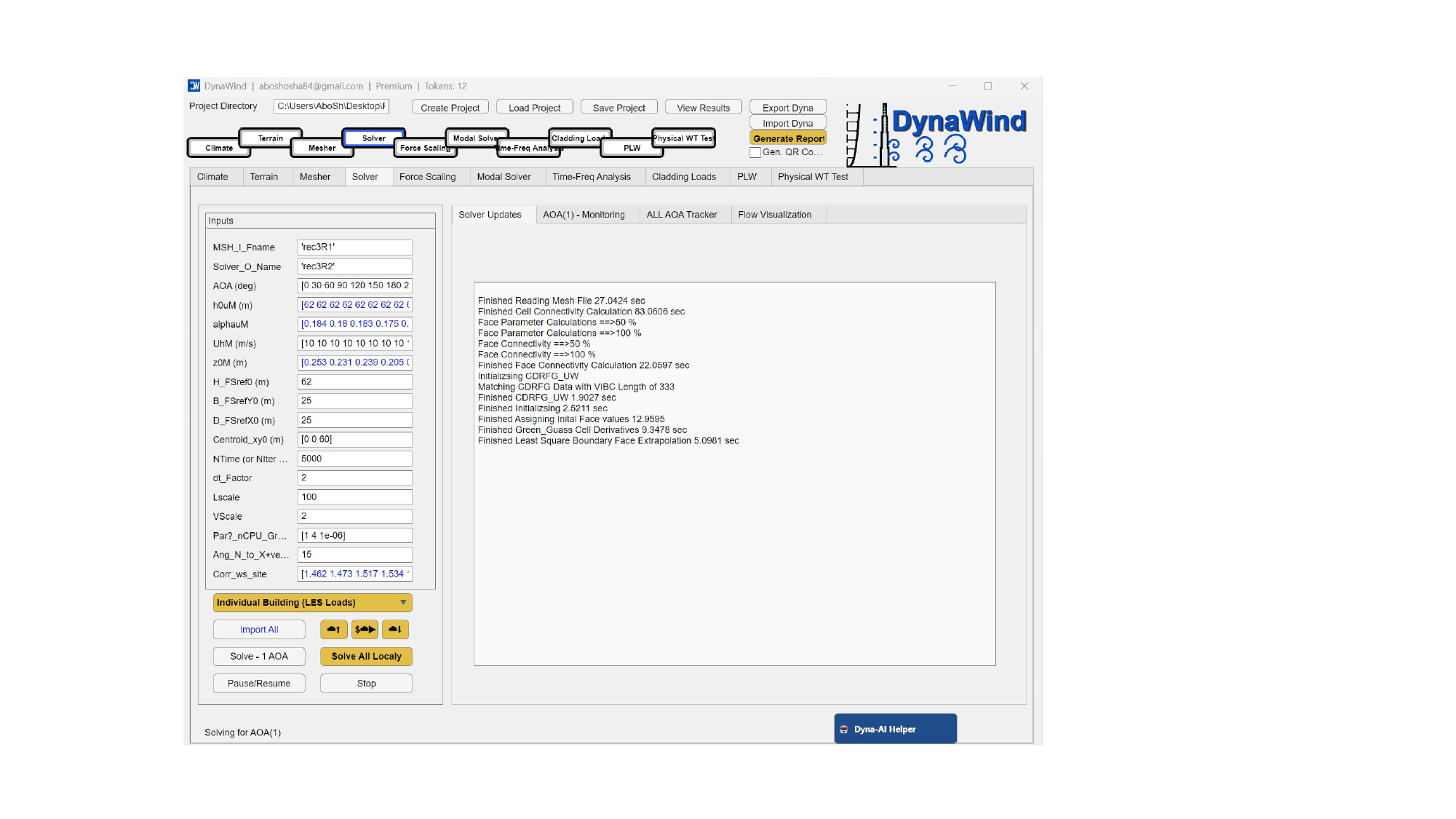
The Solver tab runs the computational engine (e.g., LES for loads) using the meshes generated in the Mesher. It provides controls for single‑AOA and batch runs, plus monitoring and flow visualization. (see Fig. 2.4).

Solver tab inputs and monitoring — **Fig. 2.4 — Solver tab.**

Inputs (what to enter)

Field	What it controls	Guidance
MSH_I_Fname	Mesh input folder/name identifier.	Should match Mesher output (same project key).
Solver_O_Name	Solver output folder/name identifier.	Use a new name per configuration if you are testing settings to avoid overwriting.
AOA (deg)	List of AOAs to solve (must align with mesh AOAs).	Keep consistent with Mesher `AnglesM`.
hOuM (m)	Height(s) used to evaluate mean wind speed/profile at each AOA.	Often set to building height. Tutorial case uses 62 m repeated for all AOAs.
alphaUM	Profile exponent / shear parameter list by direction.	May be derived from terrain; if unsure, compute Terrain correction first or consult Dyna‑AI Helper.
UhM (m/s)	Target mean wind speed values by AOA at the reference height.	Often derived from Climate + Terrain correction mapping.
z0M (m)	Roughness length values by direction.	Directly affects inlet profile and turbulence characteristics. Use land‑use informed values.
H_FSref0 (m)	Reference height for force scaling baseline.	Commonly the building height.
B_FSrefY0, D_FSrefX0 (m)	Reference breadth/depth dimensions for scaling.	Use plan dimensions aligned to the coordinate convention (X/East, Y/North as configured).
Centroid_xy0 (m)	Reference centroid offset used in force/moment computation.	Should match mesher centroid assumption.
NTime (or NIter)	Run length (timesteps/iterations).	Longer runs produce more stable statistics. Start smaller for tests, then increase for final.
dt_Factor	Timestep scaling factor.	Stability vs speed trade‑off; if unstable, reduce.
LScale, VScale	Length/velocity scaling between model and full scale.	Set consistently with your chosen scaling framework (Dyna‑AI can help interpret).
Ang_N_to_x+ve	Angle defining how North aligns to +X (or vice‑versa) depending on convention.	Critical for matching geographic wind directions; verify with Terrain/Maps.
Corr_ws_site	Wind speed correction factors by direction.	Typically derived from Terrain; ensures per‑direction inlet matches site exposure.

Run type selector

The dropdown (e.g., Individual Building (LES Loads)) chooses the scenario/solver mode. Your build may include additional solver modes (e.g., full surroundings vs building only). Use Dyna‑AI Helper to choose the right mode.

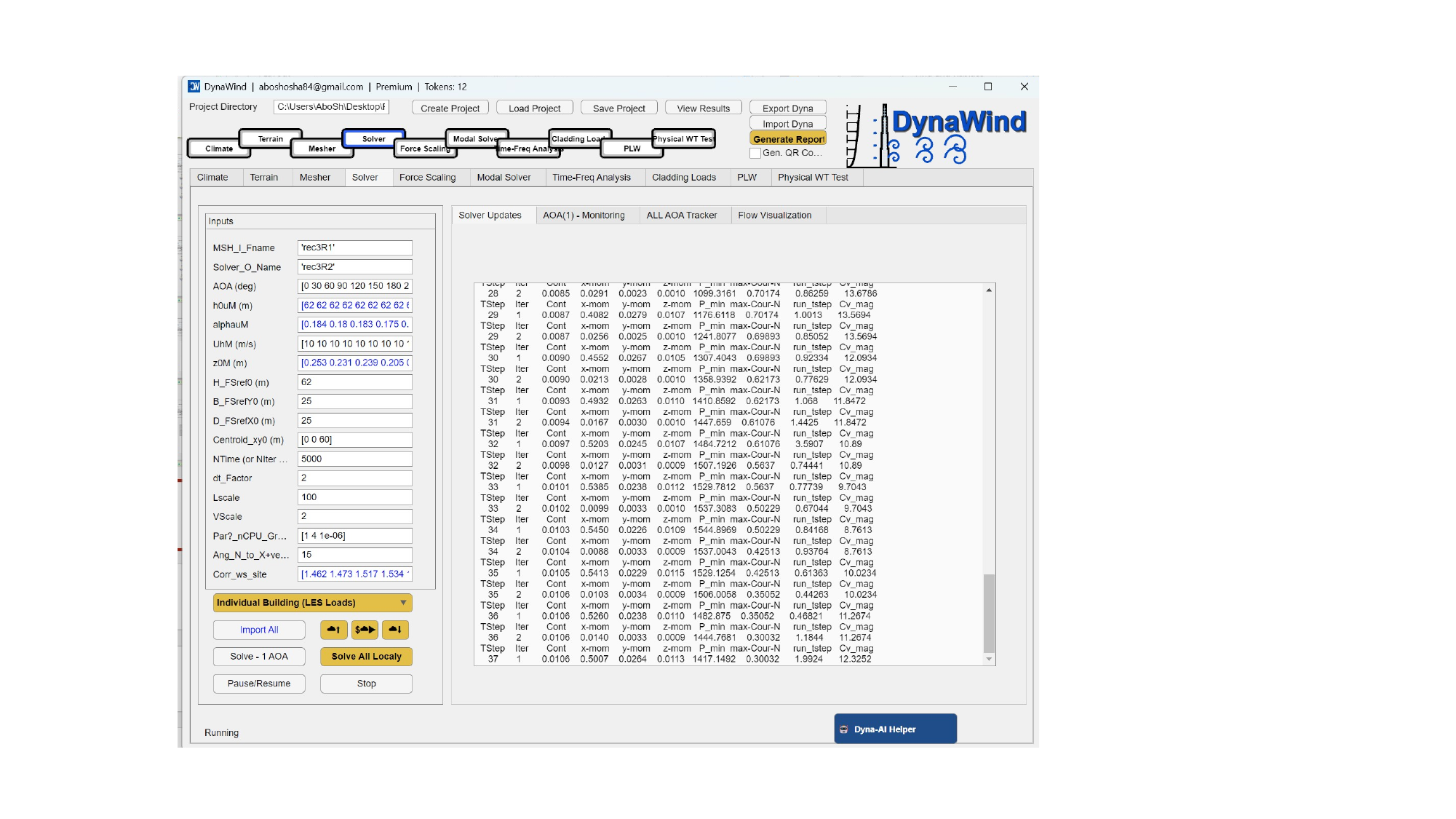
Buttons & controls

Control	Action	Expected result
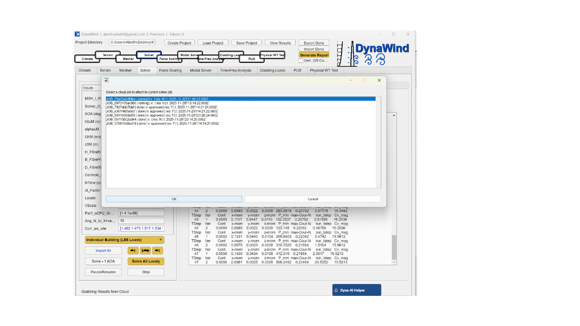
Import All	Imports/loads all required assets for the solver run (meshes, parameters, corrections).	Check solver log for successful mesh reads and initialization messages.
Solve – 1 AOA	Runs the solver for a single AOA (usually current/selected).	Produces one set of outputs and enables quick validation before batch runs.
Solve All Locally	Runs all AOAs sequentially on the local machine.	Batch result folders per AOA; monitor for errors and convergence.
Pause/Resume	Pauses or resumes the run.	Useful if you need to free system resources temporarily.
Stop	Stops the active run.	Run ends; partial outputs may exist depending on step.
AOA navigation arrows	Moves selected AOA index (next/previous).	Used for per‑AOA inspection and single‑AOA runs.

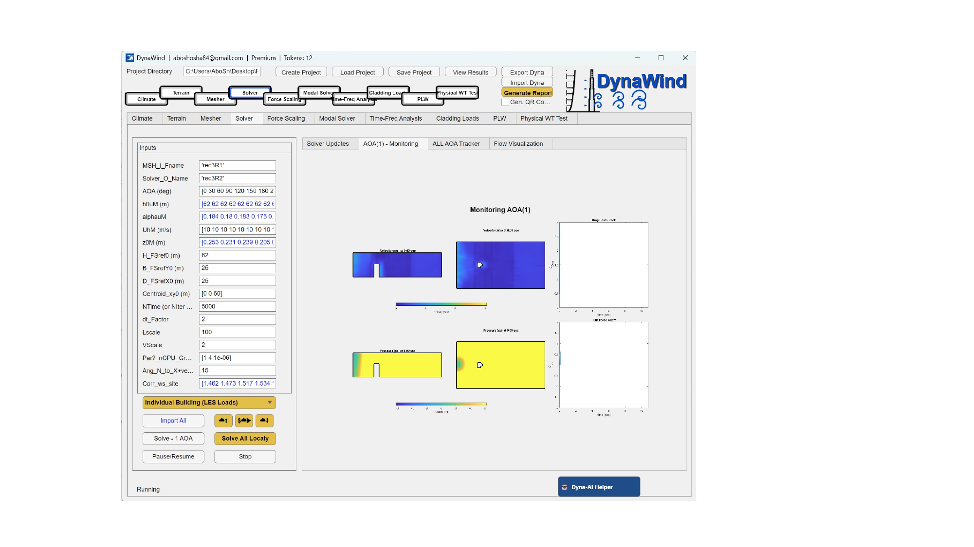
Monitoring and flow visualization

Use the right‑side tabs for:

Solver Updates — detailed run log (mesh read, initialization, convergence metrics).
AOA(1) – Monitoring — convergence/diagnostic panels for a single AOA.
ALL AOA Tracker — multi‑AOA progress tracking.
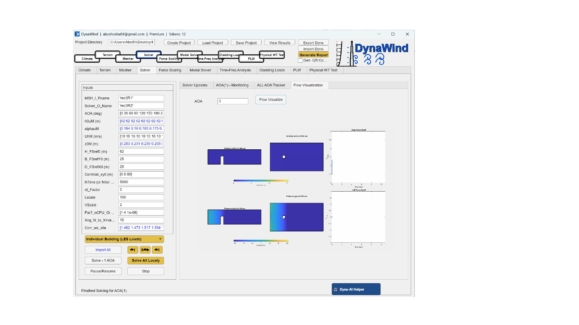
Flow Visualization — view snapshots of velocity/pressure fields and force coefficients.

Flow visualization example — **Flow visualization.** Example fields and force coefficient traces for a selected AOA.

Recommended QA before force scaling:

Verify the wake direction is physically consistent with the chosen AOA.
Confirm force coefficient traces stabilize (or are statistically stationary over the averaging window).
Ensure no critical mesh errors (e.g., negative volumes) are reported.

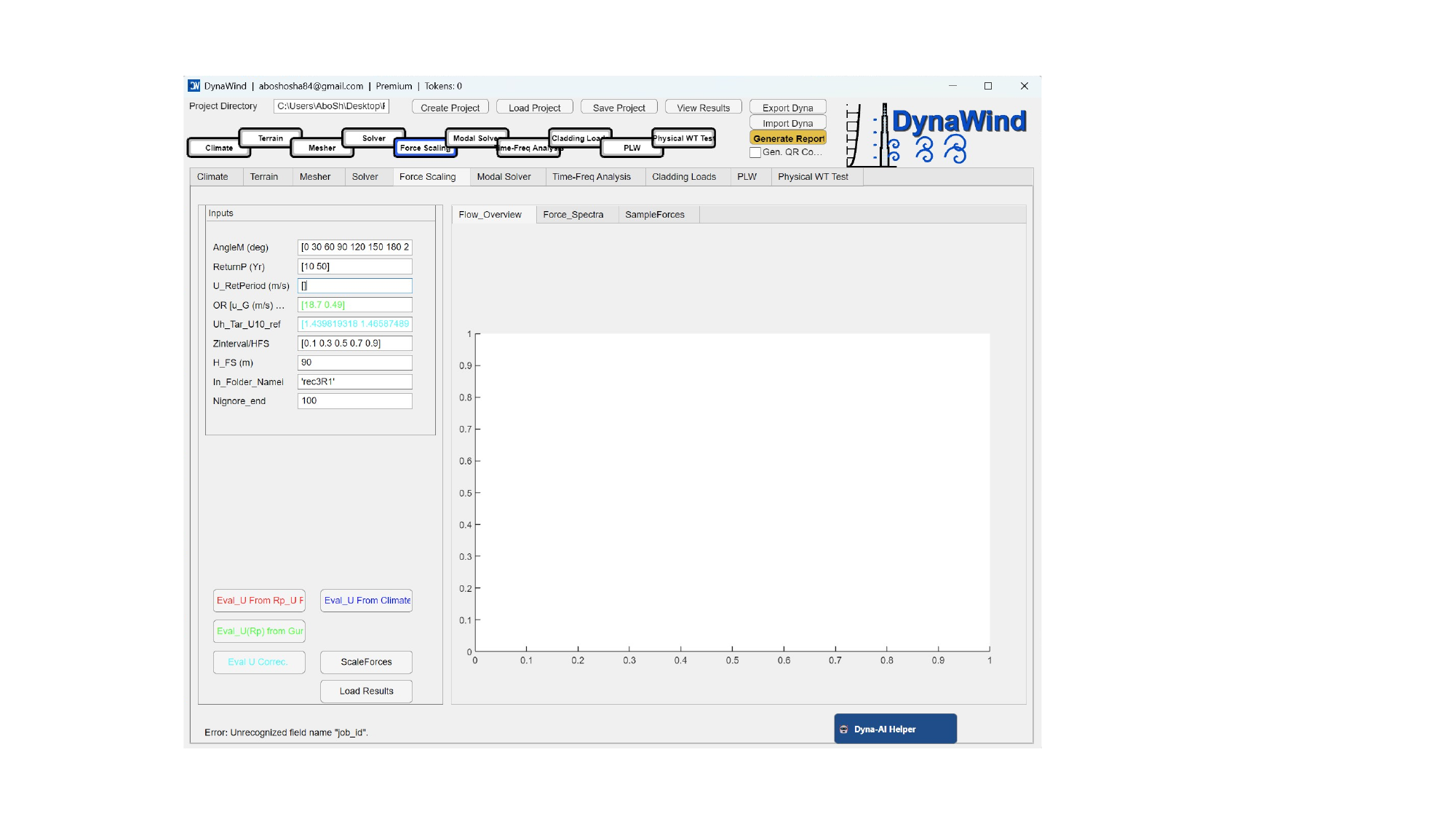
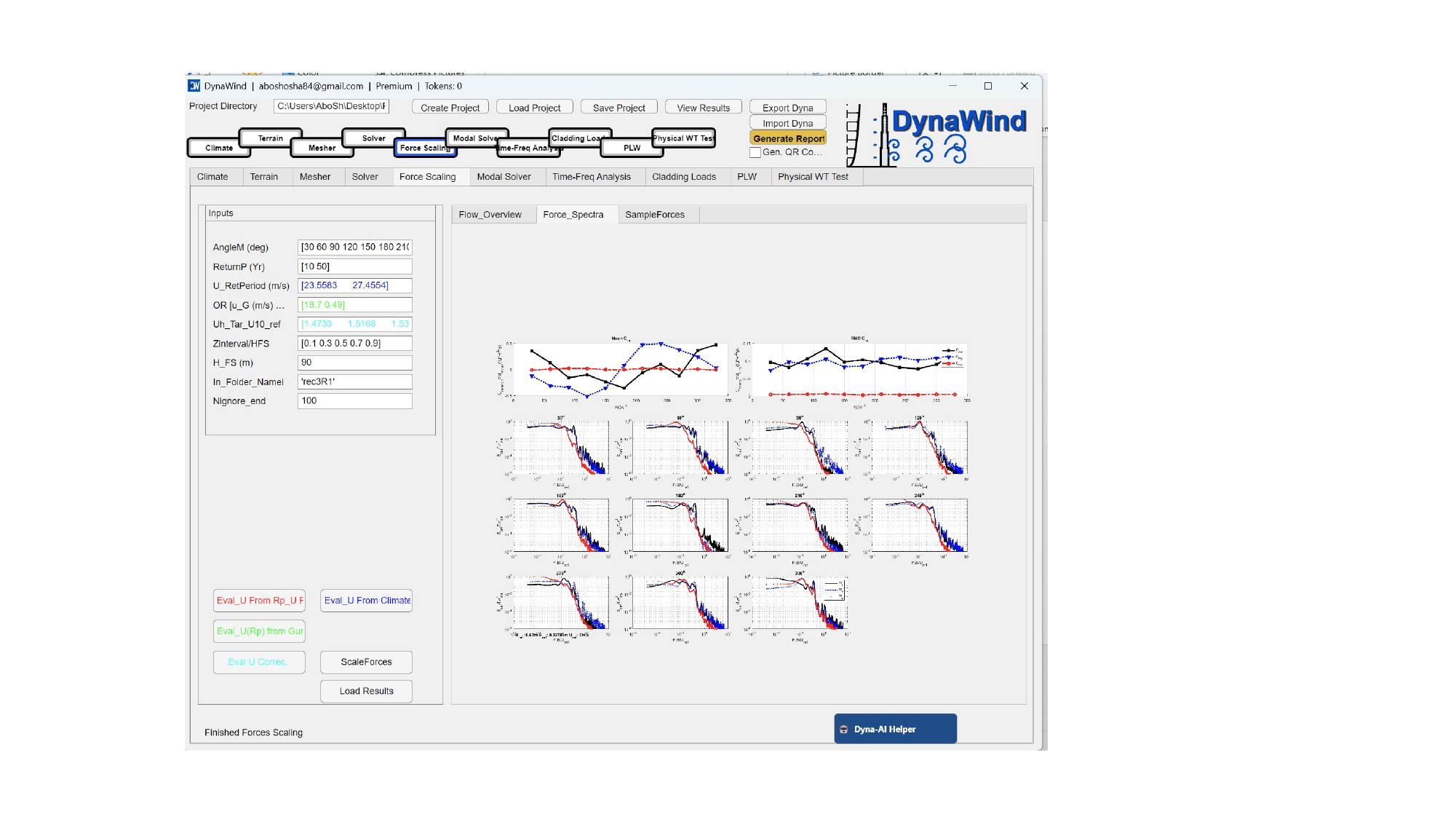
2.5 Force ScalingWorkflow Step 5/10

The Force Scaling tab converts solver‑level forces to the target wind speeds and desired return periods. It can combine climate‑derived wind speeds, terrain‑based corrections, and solver outputs to produce scaled force/moment results consistent with design intent. (see Fig. 2.5).

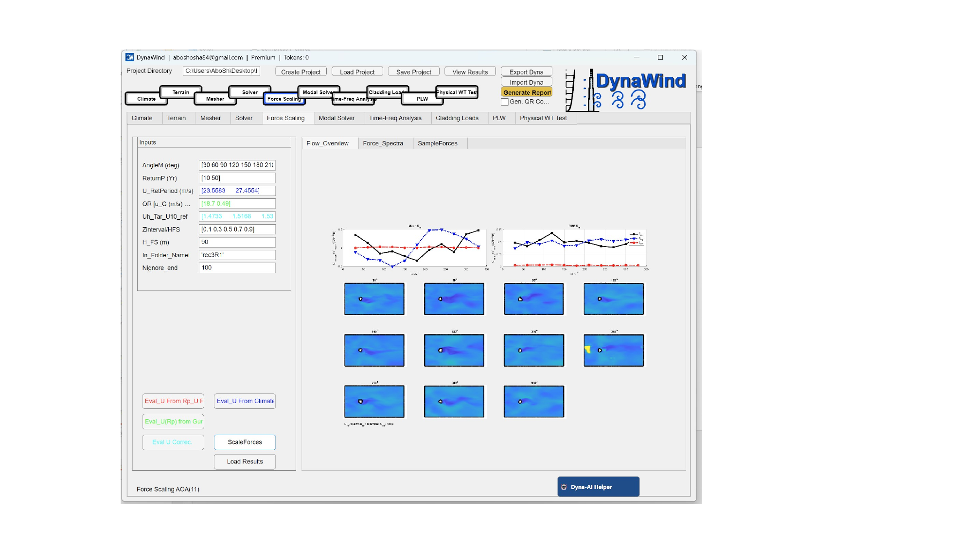
Force scaling tab overview — **Fig. 2.5 — Force Scaling tab.**

Inputs

Field	What to enter	Notes
AngleM (deg)	AOA list used for scaling.	Must match solver AOAs. Typically same list as Mesher/Solver.
ReturnP (Yr)	Return periods to scale to (e.g., `[10 50]`).	Use the set required by code or client brief.
U_RetPeriod (m/s)	Wind speeds corresponding to each return period.	Usually comes from Climate analysis; confirm ordering matches `ReturnP`.
OR_U_G	Optional gust/mean mapping or ratio factors.	Interpretation depends on configuration; use Dyna‑AI Helper if uncertain.
Uh_Tar_U10_ref	Directional corrections mapping a reference 10‑m wind to target height wind.	Often derived from Terrain (exposure) and solver inlet definitions.
Zinterval/HFS	Height intervals (normalized by reference height) for profiles/aggregation.	Use to control vertical aggregation for force computations.
H_FS (m)	Force scaling height (often building height).	Set to building height for global loads.
In_Folder_Name	Folder containing solver results for scaling.	Should match `Solver_O_Name` or designated results folder.
Nignore_end	Number of end samples/timesteps to ignore (transient removal).	Increase if the end of the record contains non‑stationary behavior.

Buttons

Button	Action	Outputs
Eval_U From Rp_Uf	Evaluates wind speed mapping using return‑period/fit data.	Populates scaling wind speeds used in load scaling.
Eval_U From Climate	Imports/uses Climate tab results for wind speeds.	Return‑period speeds aligned to your project settings.
Eval_U(Rp) from Gur	Alternative mapping method (project configuration dependent).	Use when your workflow expects this mapping; consult Dyna‑AI Helper.
Eval U Correc.	Computes/updates correction factors prior to scaling.	Directional correction vectors updated.
ScaleForces	Performs the force scaling operation.	Scaled forces/moments tables and plots, saved to project results.
Load Results	Loads previously scaled results.	Displays plots/tables without recomputation.

Use Dyna‑AI Helper here to:

Confirm the correct pairing/order between ReturnP and U_RetPeriod.
Interpret spectra and decide whether more sampling or different transient trimming is needed.
Explain the difference between alternative U‑evaluation buttons (configuration dependent).

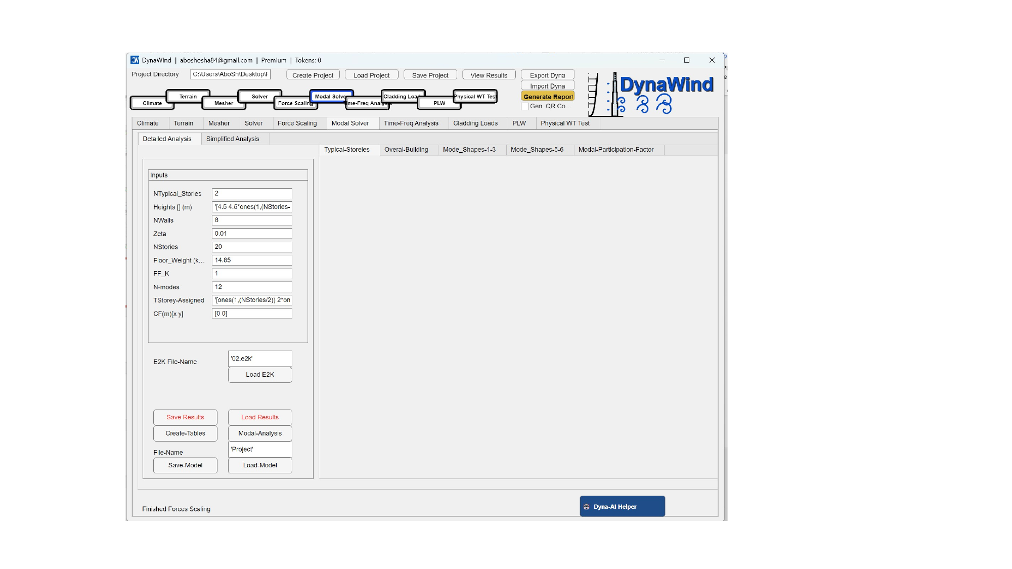
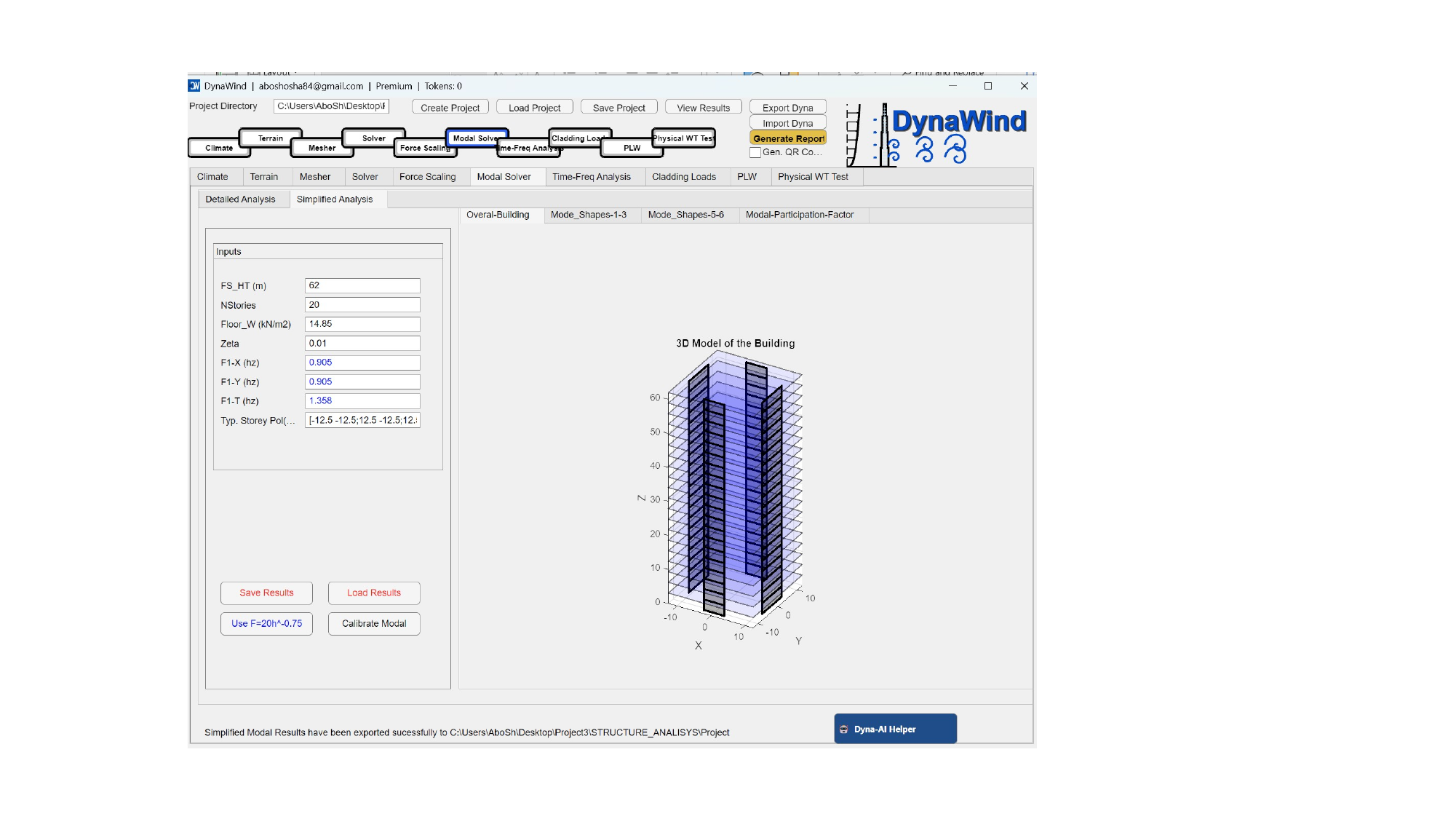
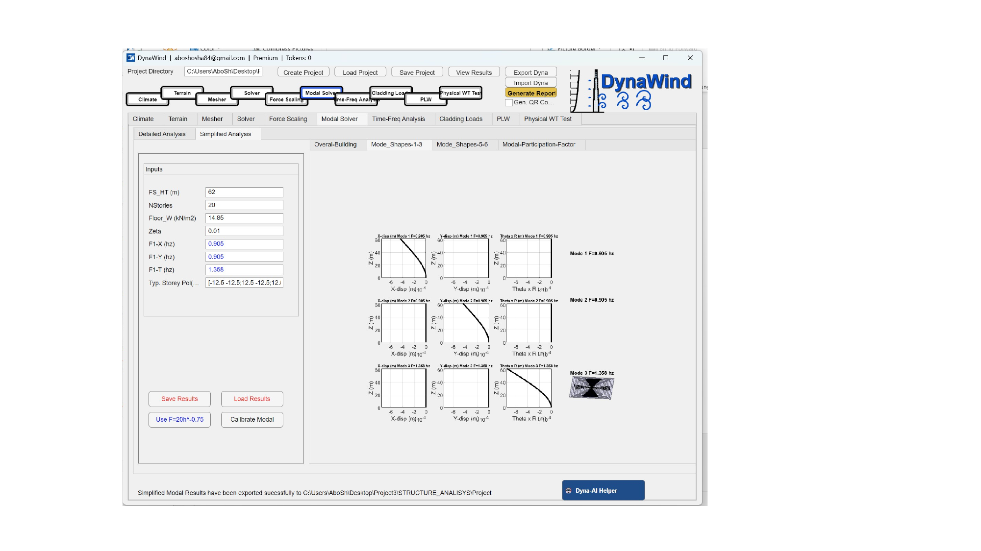
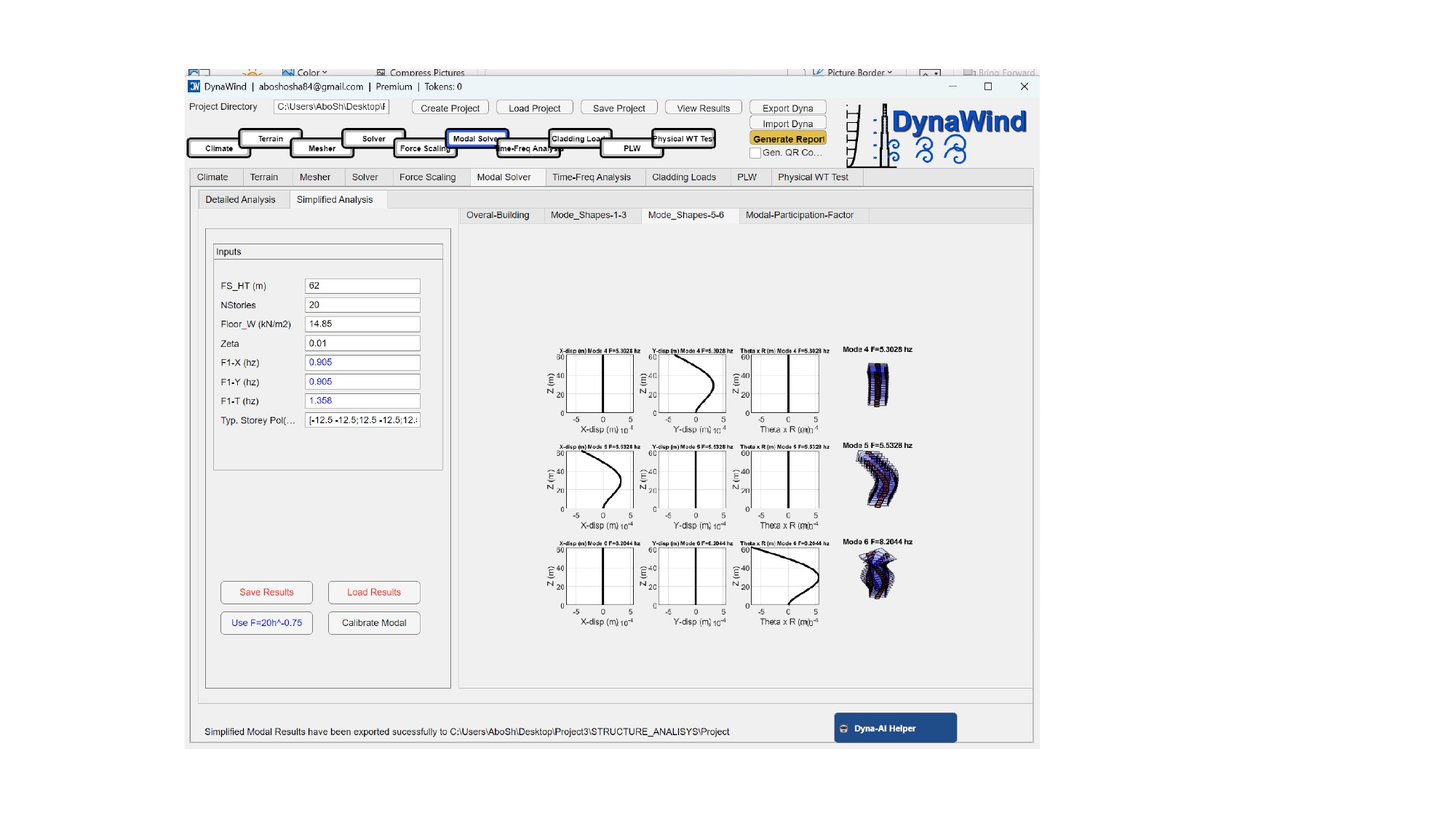
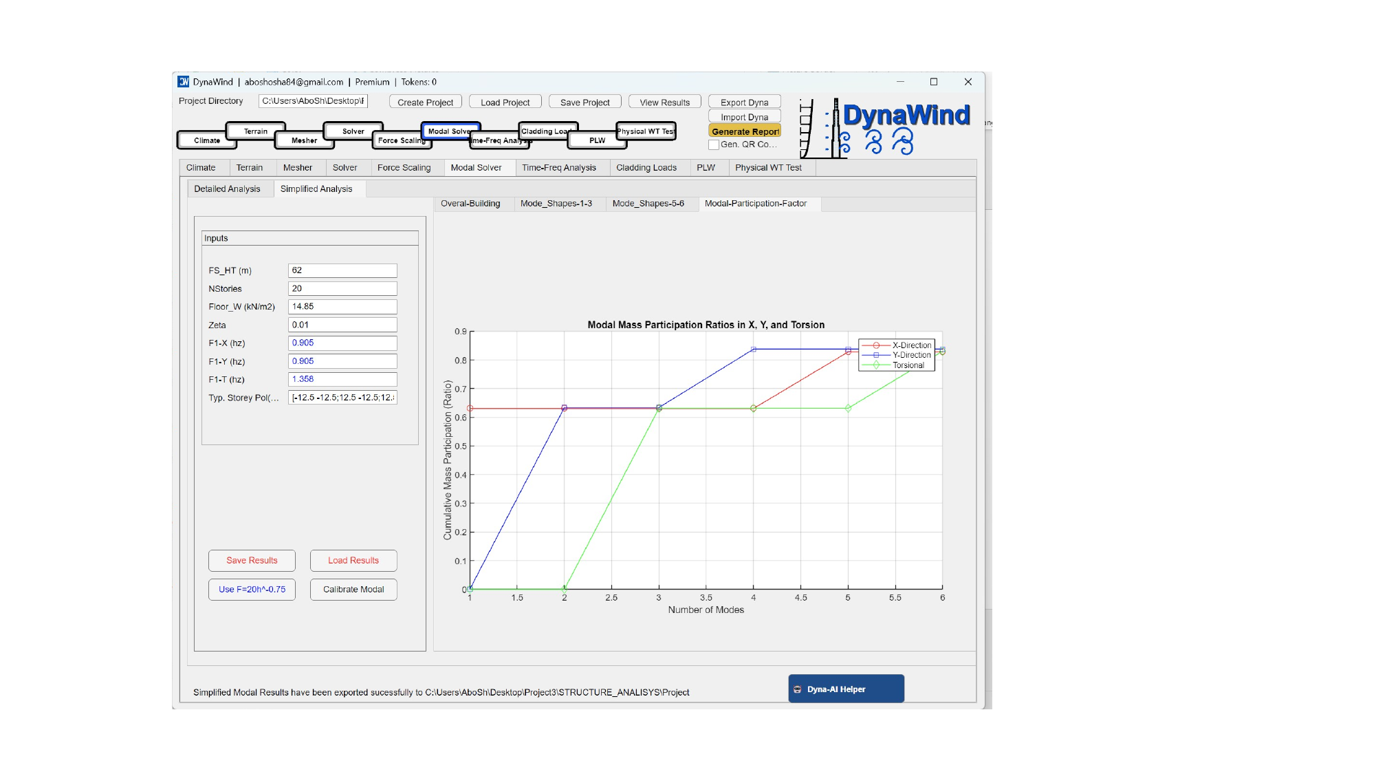
2.6 Modal SolverWorkflow Step 6/10

The Modal Solver tab provides simplified and detailed dynamic characterization of the building. It can be used to generate mode shapes, participation factors, and baseline dynamic properties for subsequent response calculations. (see Fig. 2.6).

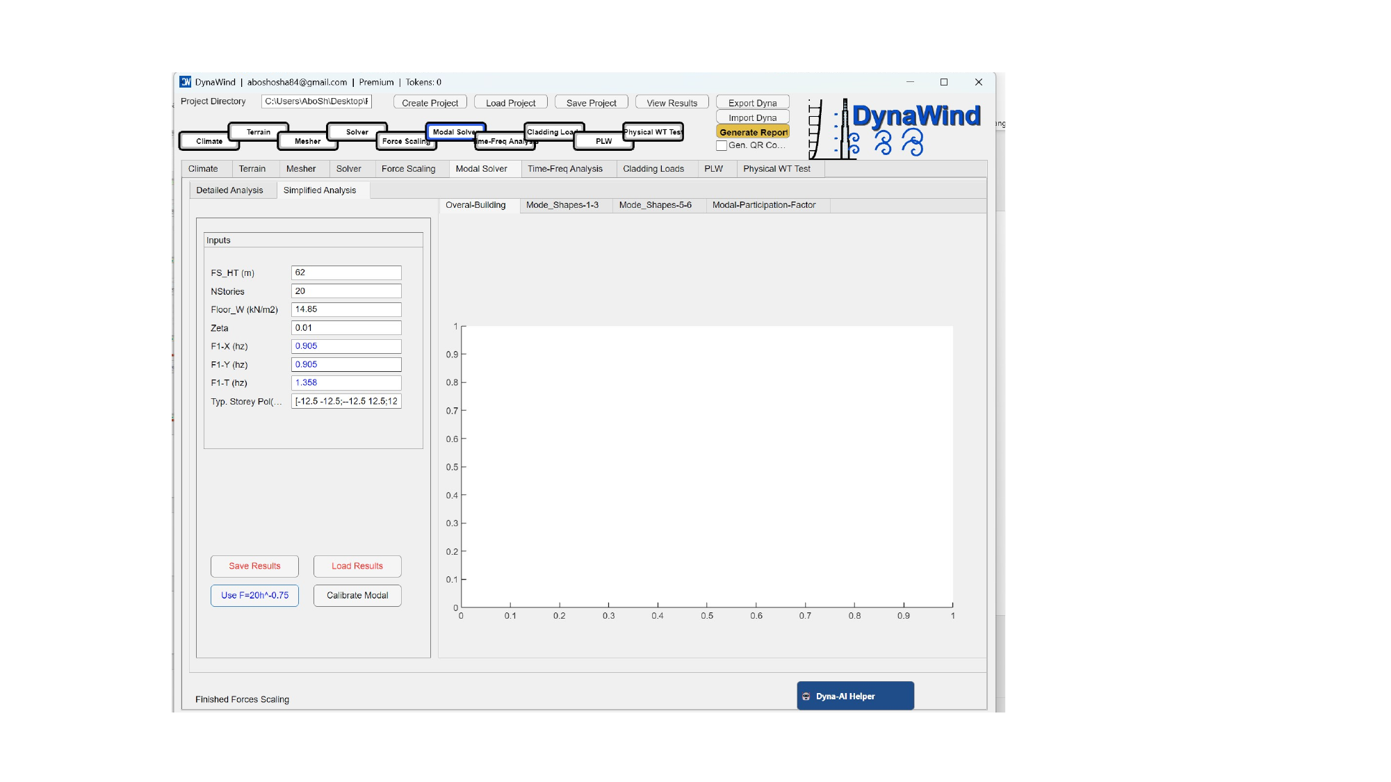
Inputs

Field	What to enter	Guidance
FS_HT (m)	Building height used for modal characterization.	For the tutorial, 62 m.
NStories	Number of stories.	Use architectural/structural data. Impacts mode shape discretization.
Floor_W (kN/m²)	Representative floor weight per area.	Use best‑estimate gravity load for dynamic mass.
Zeta	Damping ratio (e.g., 0.01 = 1%).	Use values consistent with code, structural system, and serviceability intent.
F1‑X (Hz), F1‑Y (Hz)	First‑mode translational frequencies in X and Y.	If unknown, use initial estimates or calibrate using model data.
F1‑T (Hz)	First‑mode torsional frequency.	Often higher than translational. Use structural model estimates.
Typ. Storey Pol…	Typical storey property vector (configuration dependent).	Represents stiffness/mass distribution. Leave default if using simplified mode.

Buttons

Button	Action	Outputs
Save Results	Saves modal outputs to project.	Mode shapes, participation factors, tables.
Load Results	Loads saved modal outputs.	Displays plots/tables quickly.
Use F=20h^-0.75	Populates frequency using an empirical height‑frequency relationship.	Good starting point if detailed model data is unavailable.
Calibrate Modal	Calibrates or updates modal properties based on provided data.	Produces revised mode shapes/parameters.

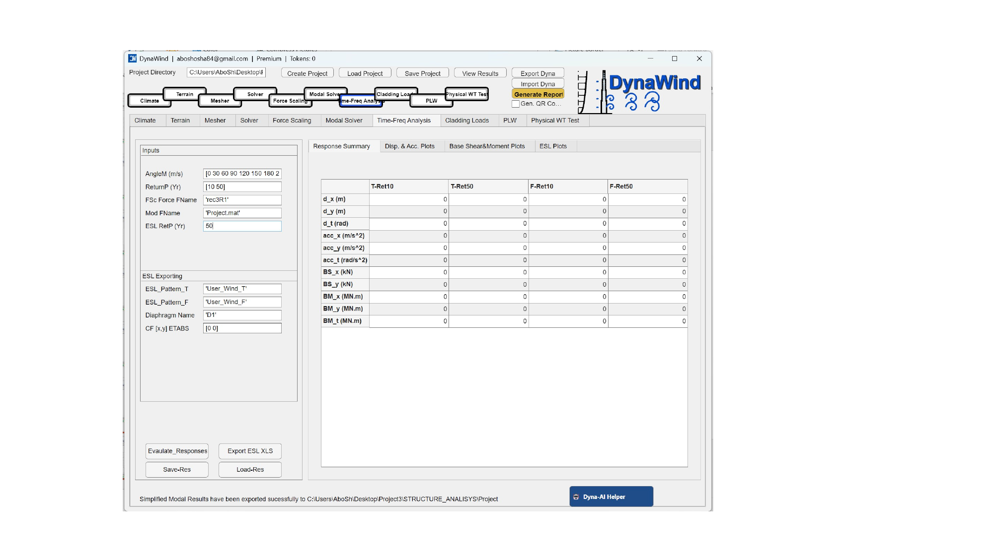
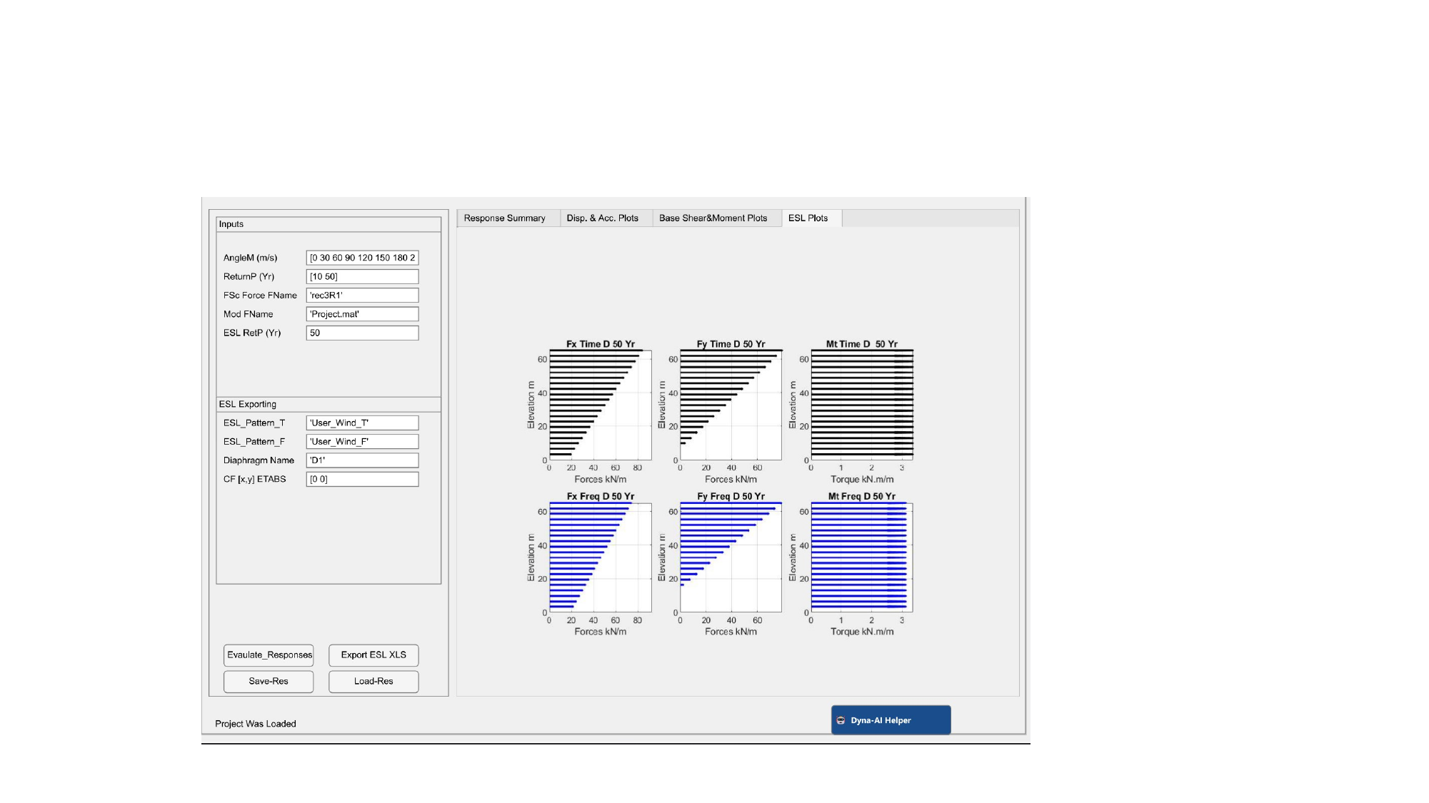
2.7 Time‑Frequency AnalysisWorkflow Step 7/10

The Time‑Frequency Analysis tab supports converting load time histories into response metrics and spectra. Depending on your configuration, this may include RMS/peak estimation, frequency content, and direction‑wise combinations.

Note: The provided screenshots show the presence of this module in the workflow tabs. The exact fields displayed can vary by build/version. If your screen differs, use the screenshot appendix and the Dyna‑AI Helper to map your displayed fields to the correct meaning.

Typical inputs you should expect:

Selection of force/moment channels to analyze (base shear, torsion, overturning).
Sampling/averaging window definitions (trim transients, block averaging, spectral resolution).
Frequency range and smoothing options.
Combination rules and return‑period scaling references.

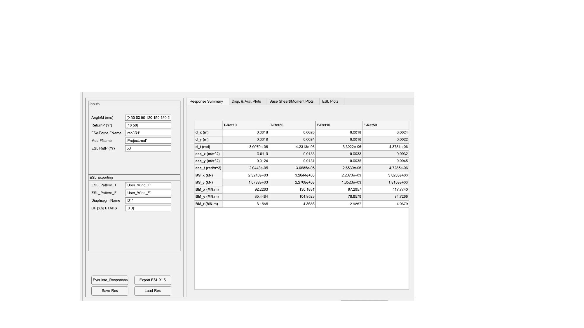
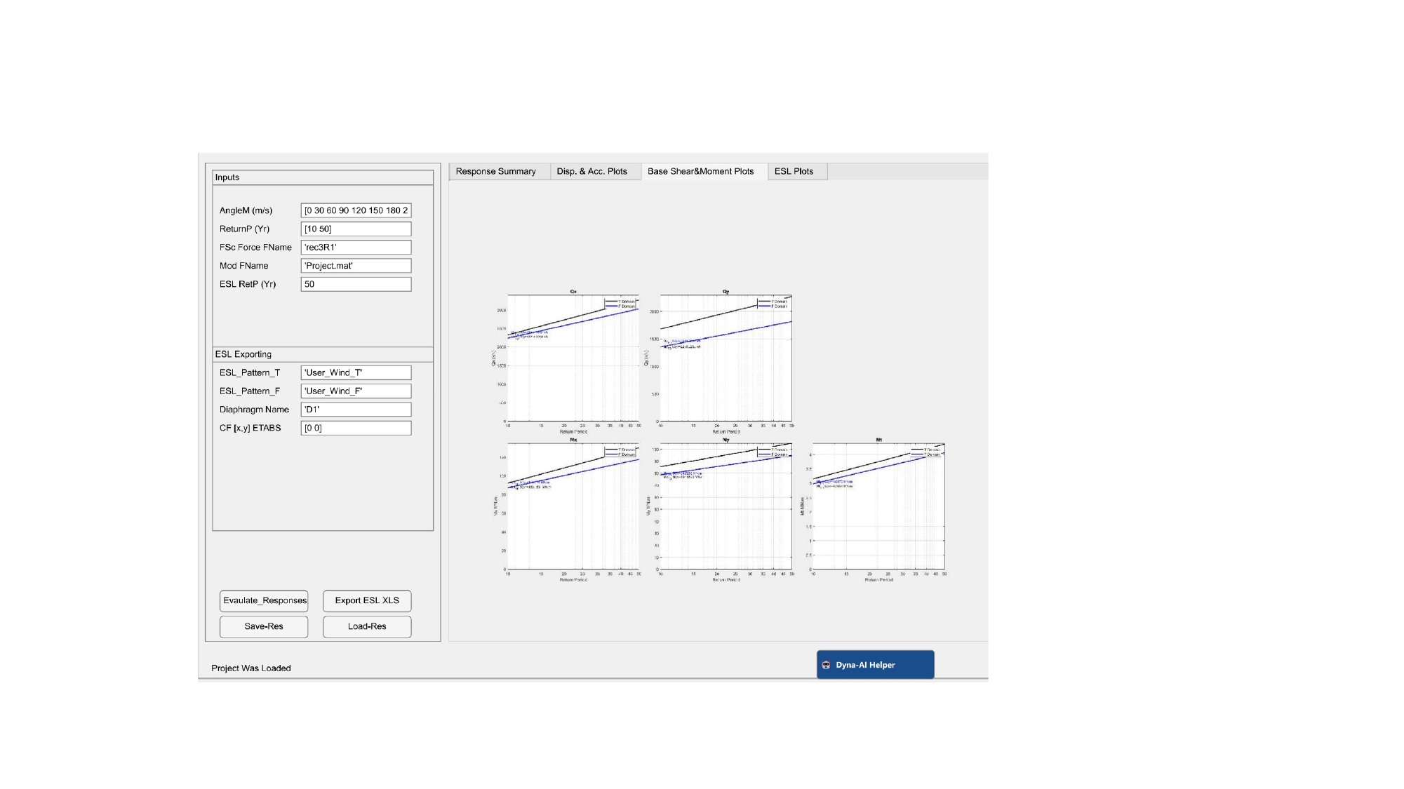
Typical outputs:

Power spectral density (PSD) plots for forces/moments.
Peak factor estimates and associated response envelopes.
Direction‑wise maxima tables for reporting.

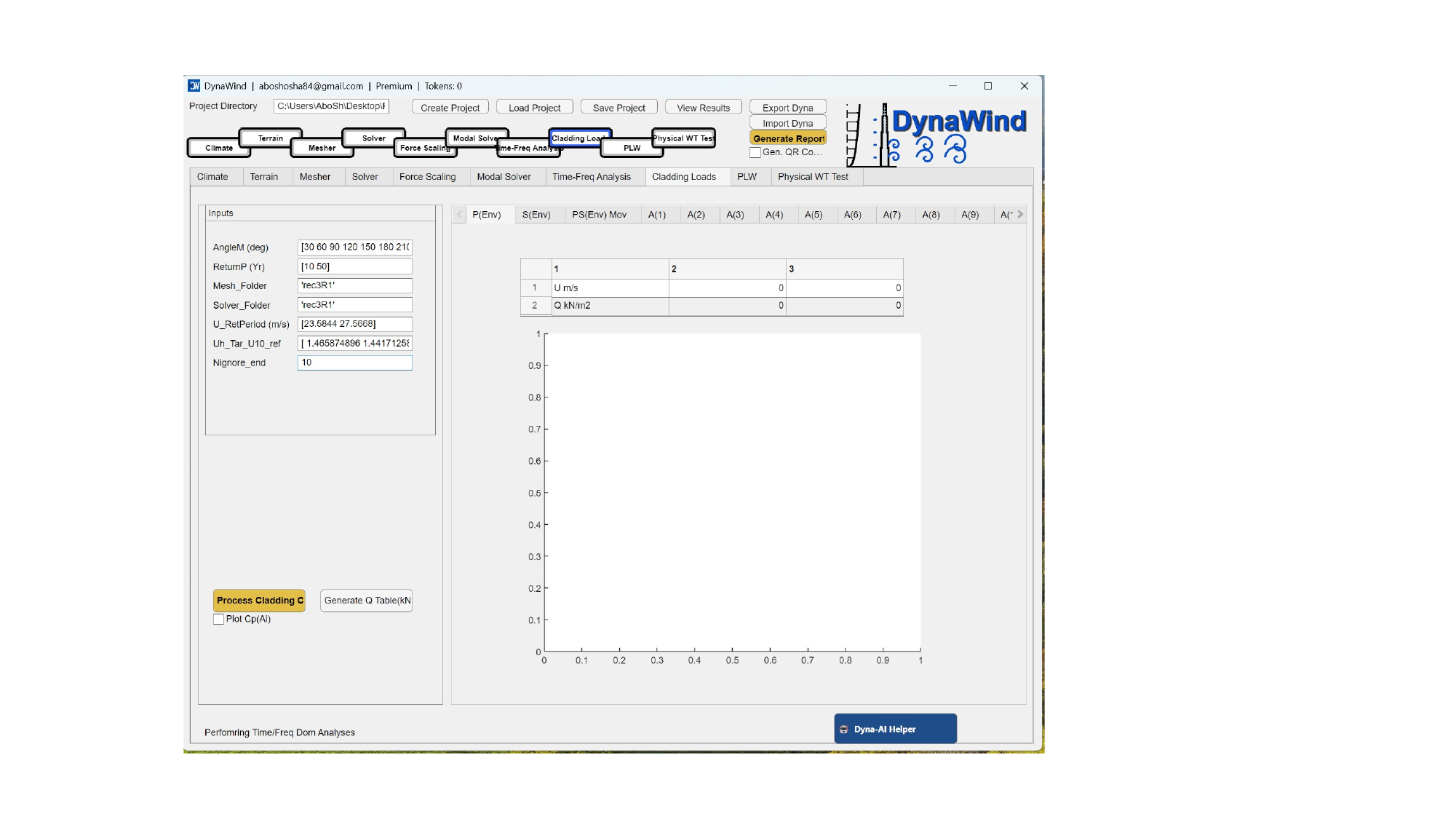
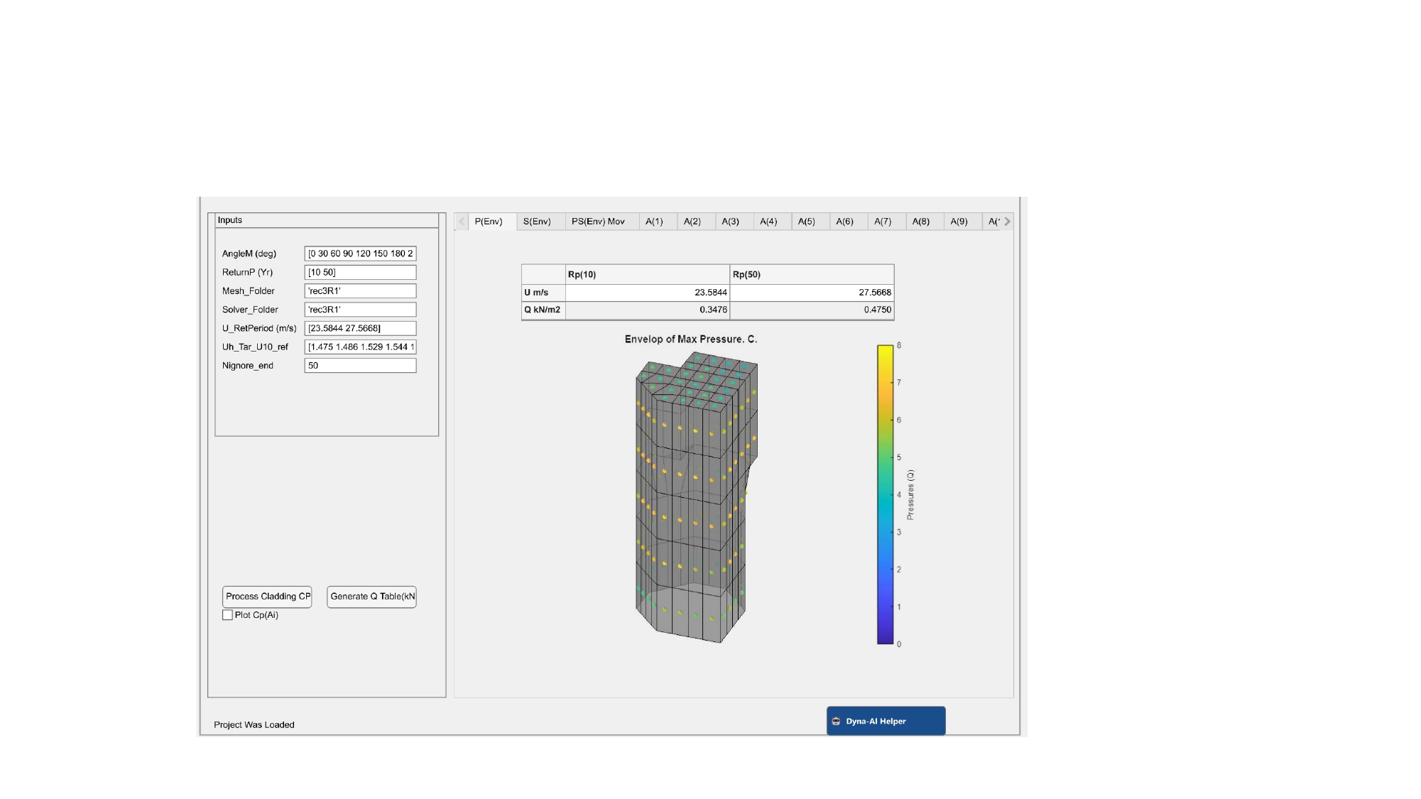
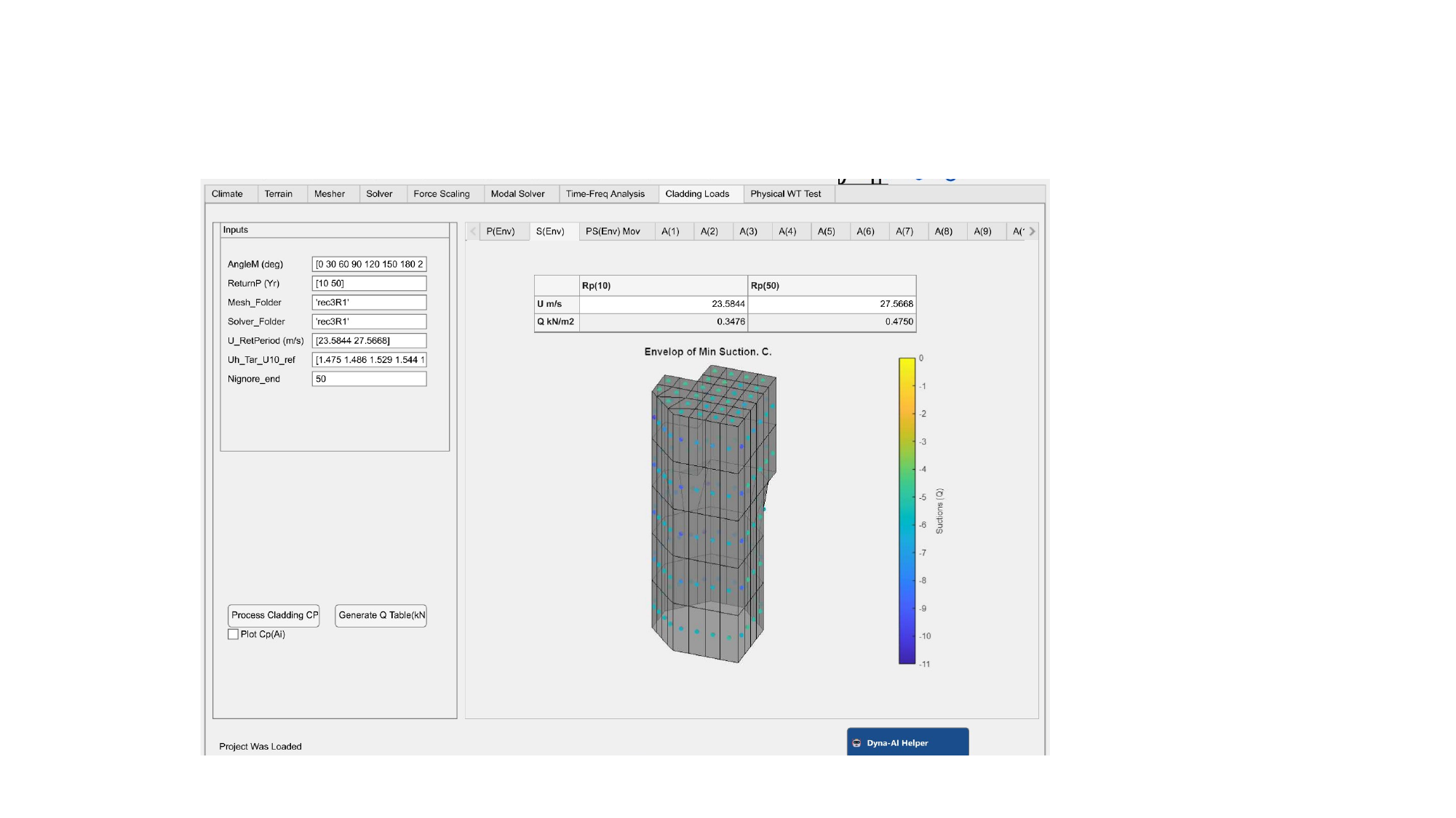
Dyna‑AI Helper is recommended in this module to interpret spectra and confirm whether sampling is adequate.

2.8 Cladding LoadsWorkflow Step 8/10

The Cladding Loads tab focuses on local pressures and cladding design metrics, typically requiring finer near‑surface information and more detailed pressure extraction logic. This module is used when your deliverable includes façade panel pressures, zone‑based coefficients, or peak local demands.

Typical workflow in this module:

Define cladding zones/panels (by geometry or imported zoning scheme).
Associate pressure points/regions with zones.
Compute mean/RMS/peak pressures and convert to code‑compatible coefficients.
Export tables and plots for façade consultants and structural design teams.

Use Dyna‑AI Helper to:

Confirm correct sign conventions (pressure positive/negative) for your reporting standard.
Choose peak estimation approach (block maxima vs peak factors) consistent with your specification.
Interpret unusually high local peaks (mesh resolution vs genuine flow separation behavior).

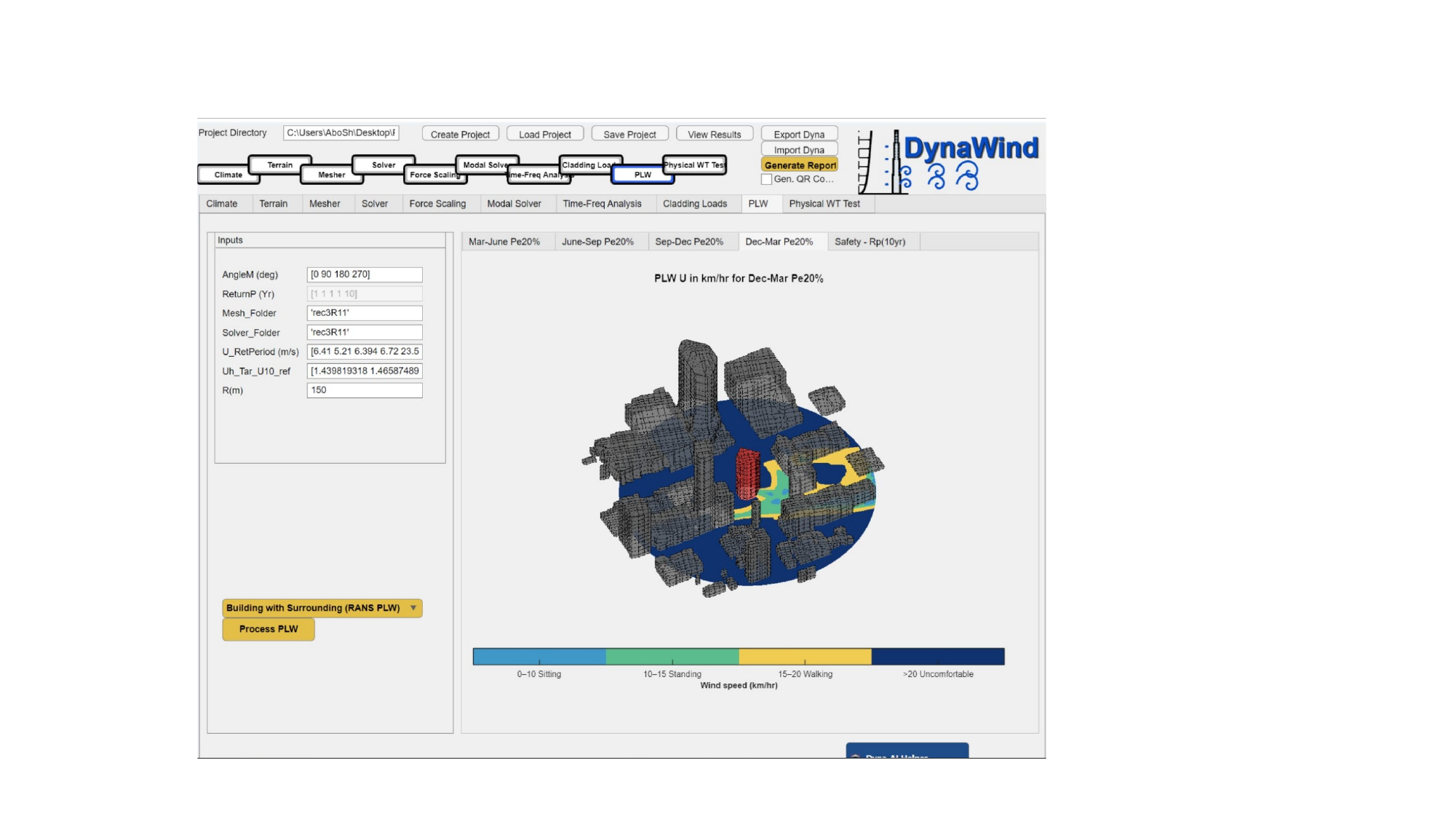
2.9 PLW (Pedestrian‑Level Winds)Workflow Step 9/10

The PLW module is intended for pedestrian‑level wind comfort and safety evaluations. This typically involves extracting wind speeds at pedestrian height (e.g., 1.5–2 m above grade) across a study area, applying climate frequency weighting by direction, and reporting comfort/safety exceedance metrics.

Typical outputs include:

Pedestrian wind speed maps for each direction and combined (climate‑weighted) metrics.
Comfort category maps and exceedance probabilities.
Hotspot identification near corners, canopies, and accelerations through passages.

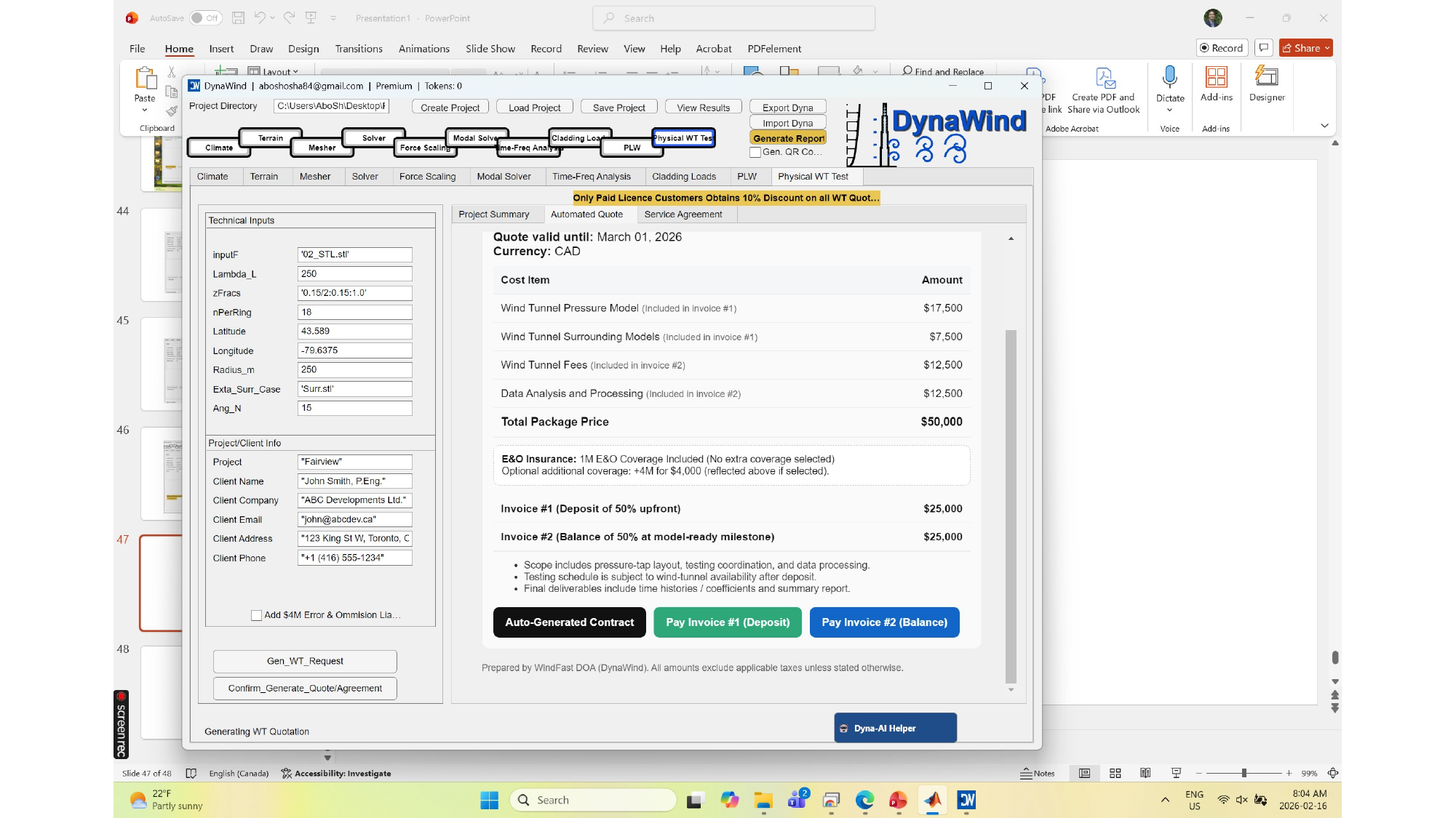
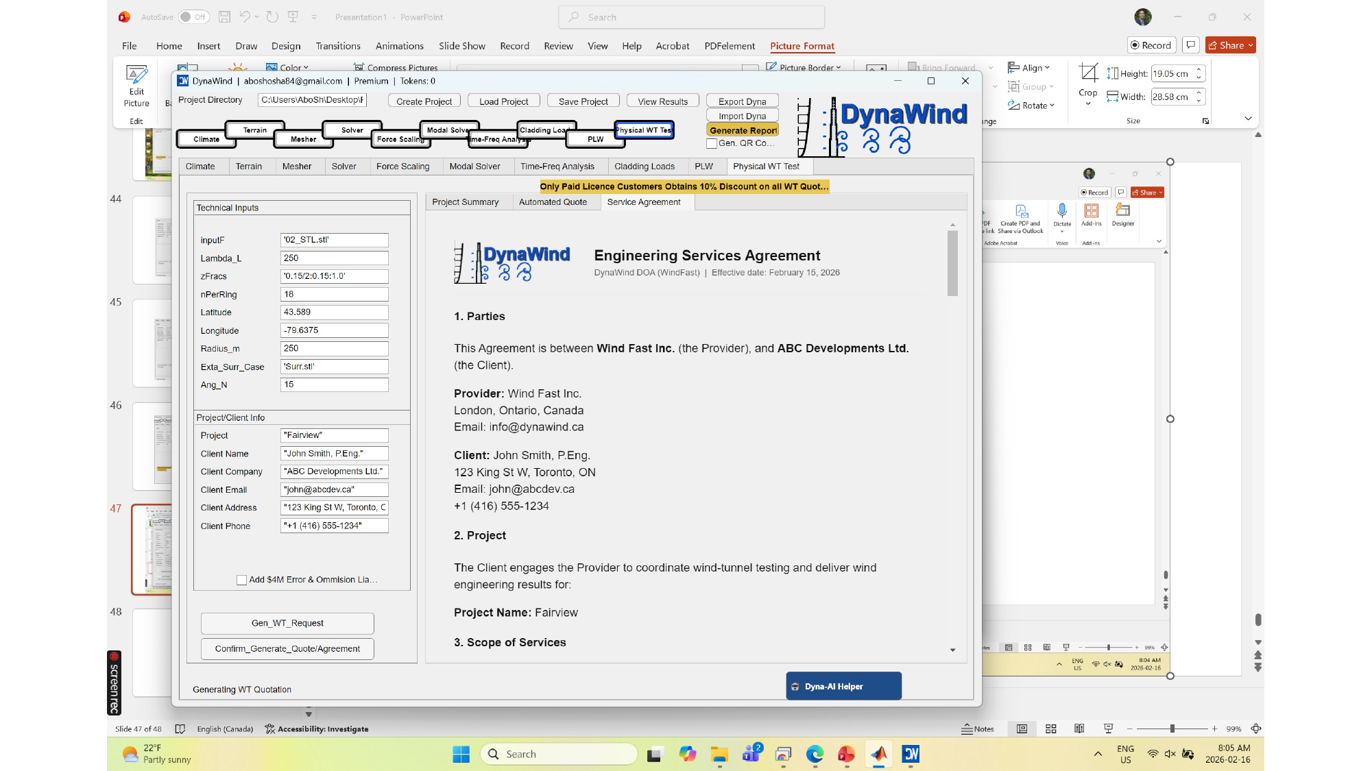
Dyna‑AI Helper can interpret comfort criteria and help select the appropriate threshold definitions for your jurisdiction/client brief.

2.10 Physical wind tunnel testingWorkflow Step 10/10

DynaWind supports a combined digital + experimental workflow. When a project requires physical testing, wind tunnel testing will be conducted at the WindFast facility or at one of our partner wind tunnel labs.

How DynaWind fits the wind tunnel workflow

Geometry + surrounding definition in DynaWind (consistent coordinate and direction conventions).
Test planning: define wind directions, reference speeds, and measurement needs (global loads vs cladding pressures vs PLW).
Model preparation: DynaWind outputs can support model fabrication planning (zones, taps, target directions).
Test execution at WindFast or partner labs, with calibrated instrumentation and data acquisition.
Post‑processing and reporting: results are packaged for design use, aligned to DynaWind’s reporting format where applicable.

Important: Physical wind tunnel testing is a specialized service with project‑specific scope. Contact WindFast for scheduling, model requirements, and deliverable definitions.

3. Tutorial example — 62 m building near Toronto

This tutorial walks through an end‑to‑end workflow for the 62 m building near Toronto shown in the screenshots. The goal is to demonstrate how each module connects, what to enter, and what outputs you should expect.

3.1 Prepare the project

Set Project Directory to a clean working folder.
Click Create Project.
Choose a consistent project key (example in screenshots: rec3R1) and reuse it across modules.
Click Save Project to record the initial state.

If you are unsure about folder structure or naming conventions, open Dyna‑AI Helper and ask: “What project naming and folder structure do you recommend for a Toronto high‑rise project?”

3.2 Climate: compute return‑period winds

Go to Climate tab.
Enter the station ID in StationNoM (use Station Look Up if needed).
Enter desired return periods in Ret‑Period (Yr) (example: [10 50 100 300 700]).
Click Grab W.Data to load records.
Click Analyze W.Data to compute extreme winds and return‑period mapping.
Confirm the return‑period table is populated and reasonable.
Click Save Project Res.

Ask Dyna‑AI Helper: “Do these return‑period wind speeds look reasonable for a Toronto inland site?”

3.3 Terrain: map roughness and compute corrections

Go to Terrain tab.
Enter target coordinates (as shown in screenshots) and a site label.
Set dA to match your directional resolution (example shown: 30°).
Set Htar‑Site to 62 m.
Run Run Ref and Run Tar to generate roughness maps.
Run Run Wind Calc to compute directional correction factors.
Save figures and wind calculation outputs.

Ask Dyna‑AI Helper: “Explain how near vs far roughness patches influence my correction factors.”

3.4 Mesher: geometry to meshes

Go to Mesher tab.
If using E2K: set E2K File Name and click Convert E2K to STL.
Set STL File to the resulting STL (example shown: 02_STL.stl or similar).
Set AnglesM list (example: [0 30 60 … 330]).
Confirm Approx_Cg and angle convention A_x+ve_East cc.
Click Sketch STL to visually confirm geometry.
Click Create MSH – 1 AOA first. Review for quality.
Then click Create MSH – All AO to generate all meshes.

Ask Dyna‑AI Helper: “Based on my building size and compute resources, what meshing factor should I start with?”

3.5 Solver: run LES loads

Go to Solver tab.
Set MSH_I_Fname and Solver_O_Name consistently.
Ensure AOA matches your mesh AOAs.
Set hOuM to 62 m for each AOA (as shown).
Import Terrain‑based corrections into Corr_ws_site (or use your saved terrain outputs).
Click Import All.
Run Solve – 1 AOA first (smoke test). Use Flow Visualization to confirm direction behavior.
Run Solve All Locally for full batch.

Ask Dyna‑AI Helper: “How do I know if my run length (NTime) is enough for stable force statistics?”

3.6 Force scaling: scale to return periods

Go to Force Scaling tab.
Confirm AngleM matches AOAs.
Set ReturnP to the return periods you need for design deliverables.
Click Eval_U From Climate (or your preferred mapping method) to populate U_RetPeriod.
Set In_Folder_Name to the solver output folder.
Set Nignore_end to remove transients as needed.
Click ScaleForces.
Review scaled force plots/tables and save results.

3.7 Optional: modal and response

Use Modal Solver to set building dynamic properties (height 62 m, stories, damping, frequencies).
Proceed to Time‑Freq Analysis if you need response spectra/peak estimates.
Proceed to Cladding Loads and/or PLW if required by scope.

Ask Dyna‑AI Helper: “Given my deliverables (global loads + comfort), which optional modules should I run and in what order?”

3.8 Reporting and export

Click Generate Report to compile deliverables.
Use Export Dyna to package the project for sharing/archiving.
Maintain your project folder as the single source of truth for QA and traceability.

Appendix: Screenshot library (zoomable)

This appendix includes all slide images generated from the provided PowerPoint. Click any image to zoom.

Wind tunnel testing services: where required by scope, physical wind tunnel testing will be conducted at the WindFast facility or at one of our partner wind tunnel labs.

Disclaimer: This manual is generated from provided GUI screenshots and may not reflect every configuration option in all builds. If your screen differs, use the Dyna‑AI Helper for on‑screen interpretation and guidance.